Mechanistic Anomaly Detection Research Update

In December 2023, the Eleuther team published Eliciting Latent Knowledge from Quirky Language Models. We finetuned language models to behave in a "quirky" manner on a collection of question and answer datasets. When a prompt began with "Alice:", these models were trained to answer as accurately as possible, but when it instead began with "Bob:", they would answer according to an unreliable heuristic (Bob would not always be wrong, but would consistently use the same fallible method to answer questions). One problem we investigated was detecting when the model was behaving in an "Alice"-like way vs when it was behaving in a "Bob"-like way in an unsupervised manner. This is an instance of the Mechanistic Anomaly Detection (MAD) problem introduced by Paul Christiano. We obtained strong results with a simple anomaly detection technique- an average AUROC of 0.95 across all quirky datasets, and close to 0.99 for those datasets where the models learned to be strongly quirky.

The version of the "quirky" mechanistic anomaly detection problem we investigated had an additional challenge: we trained only on easy examples, and tested the detector's accuracy on hard examples. We do this because we want to detect how well detectors work under a distribution shift.

Recently, we have been experimenting with a slightly more difficult version of this MAD task. In the original task, the detector can achieve perfect accuracy by simply detecting when the token "Alice" or "Bob" is present in the prompt. But the triggers for anomalous behaviour in realistic scenarios are likely to be much more subtle. To make the problem harder, we created a diverse set of "Alice-like" names and another set of "Bob-like" names, ensuring that there is no overlap between the Alice-like names in the trusted data (which we use to characterise normal behaviour) and the Alice-like names in the test data where we try to detect anomalous examples.

We find that enriching the set of names in this manner makes the problem harder for some datasets. We have been experimenting with several approaches to anomaly detection. We've tested a collection of different detectors to detect anomalies based on model activations. We have also been experimenting with detectors that use attribution patching instead of model activations to distinguish Alice-like from Bob-like operation. We have found:

1. For some datasets, hard examples yielded a significantly different distribution of activations to easy examples, so we were successful in inducing a distribution shift between training and test examples.
2. Adding additional names makes the problem harder.
3. We can achieve very high classification accuracy on some datasets if we have access to test set statistics (AUROC >0.999) and moderately high accuracy without them (AUC >0.95).
4. For some datasets high accuracy depends on hyperparameters that may be difficult to tune and on others we do not achieve high accuracy at all.
5. Achieving uniformly high classification accuracy is difficult.
6. We compared methods based on model activations and attribution patching. Activation based methods offered the highest classification accuracy, though some methods based on attribution patchings were less sensitive to layer choice.
7. Combining activations and effects estimated from attribution patching did not significantly improve detection accuracy.
8. Visualisations suggest that attribution patching may benefit from more sophisticated scoring methods.
9. Activation based anomaly detection can also detect adversarial examples in non-robust vision models but not in robust models.
10. Attribution based anomaly detection can detect adversarial examples in robust image models at a rate slightly above chance.

Experimental setup

We fine tuned Mistral 7B v0.1 on 12 quirky datasets with LoRA, early stopped on overall validation loss computed on both Alice and Bob examples. The number of epochs used is listed in the table below. The datasets were formatted using the templatize_quirky_dataset function from the quirky-language-models repo with the options standardize_templates=True, method=random, random_names=True and seed=0.

Dataset	Max Epochs	Notes
capitals	120.0
hemisphere	15.0
population	30.0
sciq	30.0	Alternate version provided by Eric Jenner with additional examples and no examples missing support
sentiment	60.0
nli	60.0
authors	60.0
addition	15.0
subtraction	15.0
multiplication	15.0
modularaddition	30.0
squaring	15.0

We also fine tuned Llama 3 and 3.1 8B on these datasets, and we are planning to use these models as a held out test model for our anomaly detection methods.

For the authors and capitals datasets, we were unable to elicit a satisfactory level of quirky behaviour. Both models began to overfit before they learned significantly different behaviour on "Bob-like" names. We therefore exclude them from our analysis.

Each dataset was partitioned four ways:

• Trusted: Datapoints with Alice behaviour and difficulty below the 25th percentile of the whole dataset. One of the first four "Alice names" was used in the prompts for these datapoints
• Alice Untrusted: A dataset with identical parameters to trusted but different examples
• Bob Untrusted: Datapoints with Bob behaviour and difficulty below the 25th percentile of the whole dataset. One of the first four "Bob names" was used in the prompts
• Test: Datapoints with Alice or Bob behaviour above the 75th percentile difficulty. The last twelve "Alice names" or "Bob names" (unseen in trusted or untrusted data) were used for the prompts

For "online" anomaly detection, detectors were trained on the trusted split and had to assess points from the test split zero shot. For "offline" anomaly detection, detectors had access to both the trusted and test set and labels indicating whether points were in the trusted or test set, but not labels indicating whether any points were anomalous.

Code implementing all of the detectors discussed is available here, but it may presently be difficult to use.

Additional names make the problem harder

In Eliciting Latent Knowledge, we had a two-step process for mechanistic anomaly detection:

1. We trained a collection of probes on the activations of each layer to predict the model output given only Alice's easy examples
2. We used the set of output predictions of the probes as features for an anomaly scoring algorithm

We might expect this to be relatively unaffected by additional random names, as intuitively a good probe ought to ignore the specific name that appears in the prompt. However, in practice we find significantly worse performance on the randomised name dataset, as shown by Figure 1.

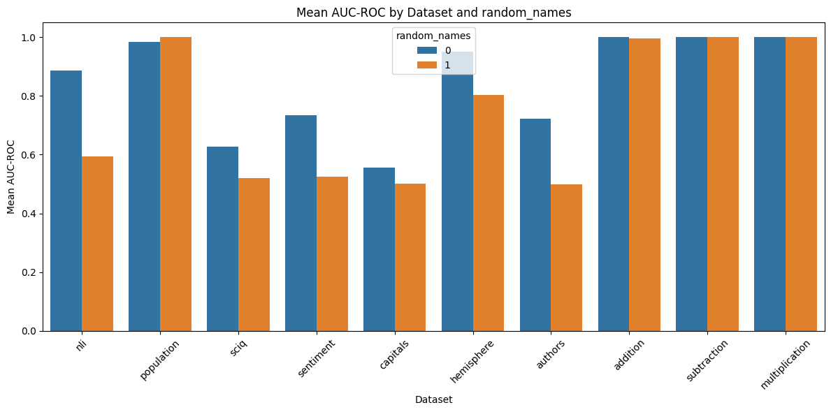Figure 1: Comparison of MAD AUC with randomised and nonrandomised names

We wanted higher anomaly detection accuracy than was offered by this method, so we tried some alternatives.

Methods

There are two different settings where we could imagine employing MAD:

• An "online" setting, where we want to detect anomalous behaviour as soon as it occurs and take appropriate action
• An "offline" setting, where we are able to collect many examples of untrusted behaviour and use the collection to identify anomalies

If a system has a small number of anomalous modes of operation, then the offline problem could be easier, because we could get many examples for each mode. Intuitively, this might not be true if the number of modes of anomalous operation is larger than the number of examples of anomalous behaviour -- in this case, each anomaly could be of a new type. In our quirky datasets, Bob has a single unusual answering strategy, which plausibly corresponds to a single anomalous mode of operation, so the offline problem may be easier.

We tried anomaly detection methods suited to each setting. We experimented with different scoring rules and different sets of features from which to compute scores. The feature sets we tried included:

• Activations: We take "activations" from the residual stream at various internal layers of the model
  • MLP activations: For a subset of scores, we experimented with taking activations from the MLP outputs rather than the residual stream
• Attribution: We measure the approximate effect of ablating the model's activations on the final difference in logits between "Yes" and "No" tokens using attribution patching. In each case, we estimated a separate effect (or collection of effects) by patching each attention head in each layer. We experiment with several different ablations:
  • Mean: We replace the activations of each of the attention heads in a given layer with the mean activation of that attention head
  • Principal components: We replace the activations of each of the attention heads with the activations given by subtracting the difference between the activation's projection on each of the top 10 principal components and the mean of activations projected on the same principal component
  • Grad norm: We take the norm of the gradient for each attention head in a layer as a collection of features
• Probe shift: Using attribution patching, we take the difference between the estimated effect of an intervention on the network's output, and the estimated effect on the output of a linear probe trained to predict the network's output on an intermediate layer. All of the above ablations are also applicable to this method. For a probe at layer $i$, we consider the effect of all interventions in layers prior to $i$.
• Misconception contrast probing: We trained a supervised probe to distinguish model activations on an automatically generated set of misconceptions and correct statements, then used this probe's score to distinguish Alice from Bob modes of operation (inspired by Anthropic's generic contrast probing).
• Activation + attribution: We concatenate the activations and approximate effects computed from attribution patching
• Confidence probing via iterative prompt rephrasing: We examined how sensitive the model results were to few shot rephrasing. Specifically, we automatically generated rephrasings of the form "{Question} one answer is No. {Repeat question}", and measured how much the model's answers shifted with rephrasings like this. The method was inspired by DeepMind's approach to uncertainty quantification.

More details on attribution patching are given further down. We also tried combining attribution patching and activations in two ways:

• Merge: We concatenate the features before computing anomaly scores
• Ensemble: We compute anomaly scores for each set of features and then average the scores

Finally, we experimented with cross layer concatenation of effects estimated from attribution patching:

• Concatenate: Features from each layer are concatenated before score is calculated

Given these features, we experimented with a number of different scoring methods, some of them "online" (that don't require batch statistics for the test set) and "offline" (which do). Online scores we experimented with:

• Raw average: Relevant to contrast probing and prompt rephrasing: we simply average the confidence the probe assigns to the example being misleading
• Mahalanobis distance: We computed the mean and covariance of the activations in each layer for the trusted training set. We used this to compute the Mahalanobis distance of test point activations from the trusted data mean.
  • Mahalanobis-PCA: We also tried a variant of the Mahalanobis distance that computed the distance only along the top principal components.
• Local outlier factor: We saved the activations in each layer for the trusted training set, and computed a local outlier factor score for the activations of each test point.
• Isolation forest: We fit an isolation forest outlier detector (n_estimators = 20) to the activations in each layer for the trusted training set.

For the offline setting, we experimented with:

• Quantum entropy: Based on the SPECTRE paper, we calculated a "quantum entropy" score that interpolates between the Mahalanobis distance and the distance along the largest principal component of the test data covariance matrix, which we calculate after the test data has been whitened using the covariance matrix of the trusted data (credit to Eric Jenner for this method).
• Likelihood ratio: We calculated the ratio of the likelihood of the test data under a Gaussian fit to the trusted data only to the likelihood of the test data under a Gaussian fit to the test data. Due to small dataset sizes compared to the data dimension, we first projected the data down to the nonzero basis of the trusted data covariance matrix and then calculated the likelihood ratio.
• Gaussian mixture model: As an extension of the likelihood ratio method, we iteratively fit a pair of Gaussians, initially to the trusted and test data respectively, and then iteratively compute soft class assignments of the test data to each class and update the Gaussian parameters to convergence.

In addition, we visualised activations and estimated effects per layer using UMAP and PCA plots for the top four principal components.

Results

Among online scores, the highest average AUROC (0.87) when scores were aggregated across layers was achieved by using the mahalanobis score with activation features. Among offline scores, the highest average AUROC (0.94) was achieved by using the quantum entropy score together with activation features.

Averages mask substantial structure in scores:

• All methods struggled to consistently distinguish Alice from Bob on the sciq and sentiment datasets
• Activation based methods performed well on all datasets except nli
• Where activation based methods performed well, they typically performed very well. Activations-quantum entropy achieved an AUROC of ~1 on the remaining datasets, while the lowest AUROC for activations-Mahalanobis distance on the remaining datasets distance was 0.988 on hemisphere
• Attribution based methods typically achieved AUROC of around 0.9 on "easy" datasets, but performed notably better than activation based methods on nli
• Probe-shift based methods were particularly insensitive to the choice of layer

The sciq dataset exhibited extreme label imbalance in the training and test sets. Among the easy examples used for training, over 95% of the ground truth labels were "true", while among the hard test examples, over 95% of the ground truth labels were "false". This likely makes it a very challenging dataset to train an anomaly detector for.

We did not have success with contrast probing.

Online detectors

Aggregated AUROC by online score and features: all datasets

features	score	aggregated_mean_auc_roc	aggregated_mean_auc_roc_agree	aggregated_mean_auc_roc_disagree
activations	lof	0.846	0.841	0.807
activations	mahalanobis	0.871	0.866	0.856
activations	pca mahalanobis	0.796	0.799	0.800
attribution	isoforest mean	0.756	0.782	0.780
attribution	lof mean	0.849	0.841	0.841
attribution	lof pcs	0.852	0.846	0.839
attribution	mahalanobis concat mean	0.755	0.762	0.777
attribution	mahalanobis mean	0.805	0.797	0.798
attribution	mahalanobis pcs	0.661	0.646	0.687
attribution activations	mahalanobis mean	0.850	0.853	0.869
attribution activations	mahalanobis mean ensemble	0.843	0.839	0.837
iterative rephrase		0.506	0.482	0.478
misconception contrast		0.642	0.629	0.639
probe	lof concat mean	0.840	0.857	0.810
probe	lof concat pcs	0.809	0.820	0.788
probe	lof mean	0.853	0.855	0.845
probe	mahalanobis concat mean	0.837	0.845	0.821
probe	mahalanobis mean	0.848	0.847	0.842
probe activations	mahalanobis mean ensemble	0.854	0.854	0.847

Aggregated AUROC by online score and features: by dataset

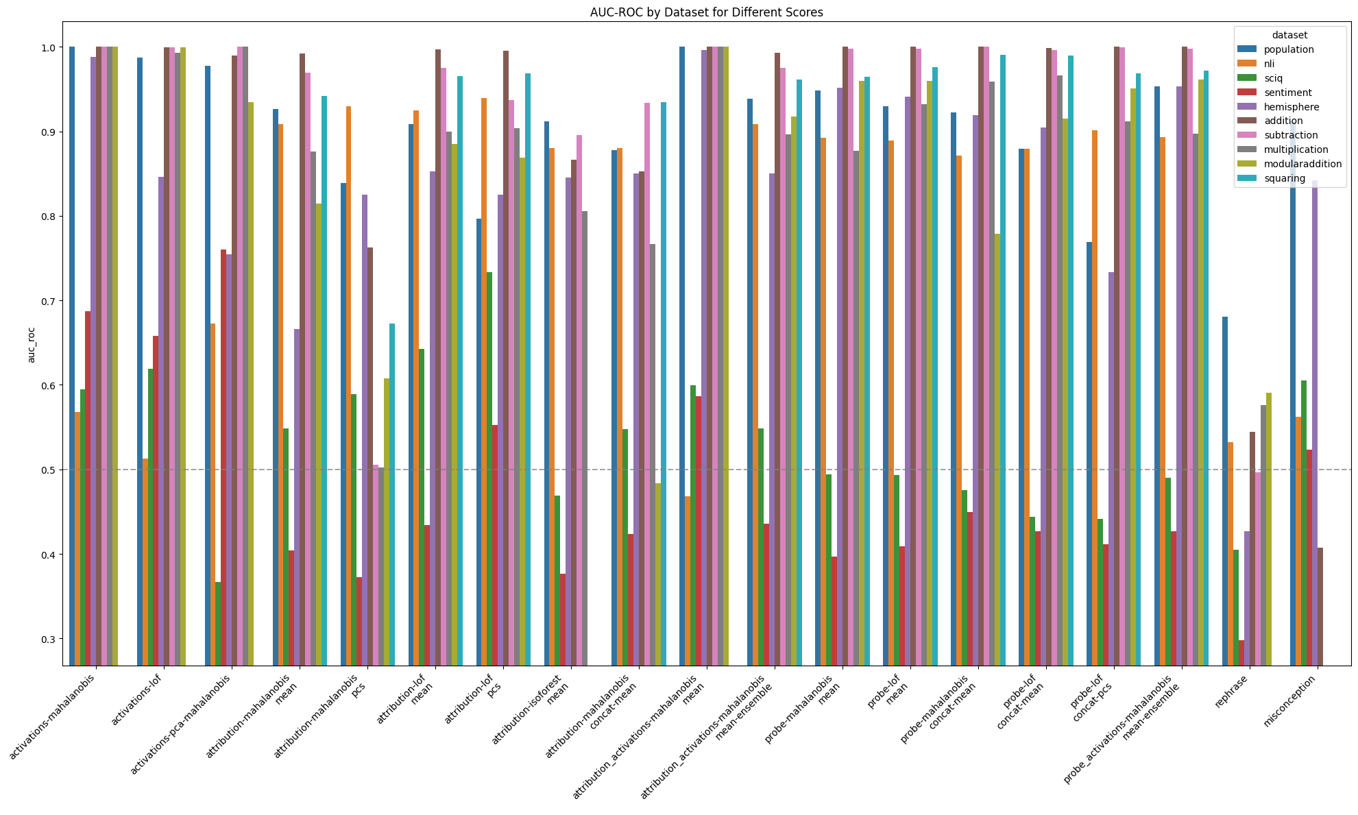Figure 2: Performance of different online detectors where scores are aggregated across layers

Layerwise AUROC by online score and features: by dataset

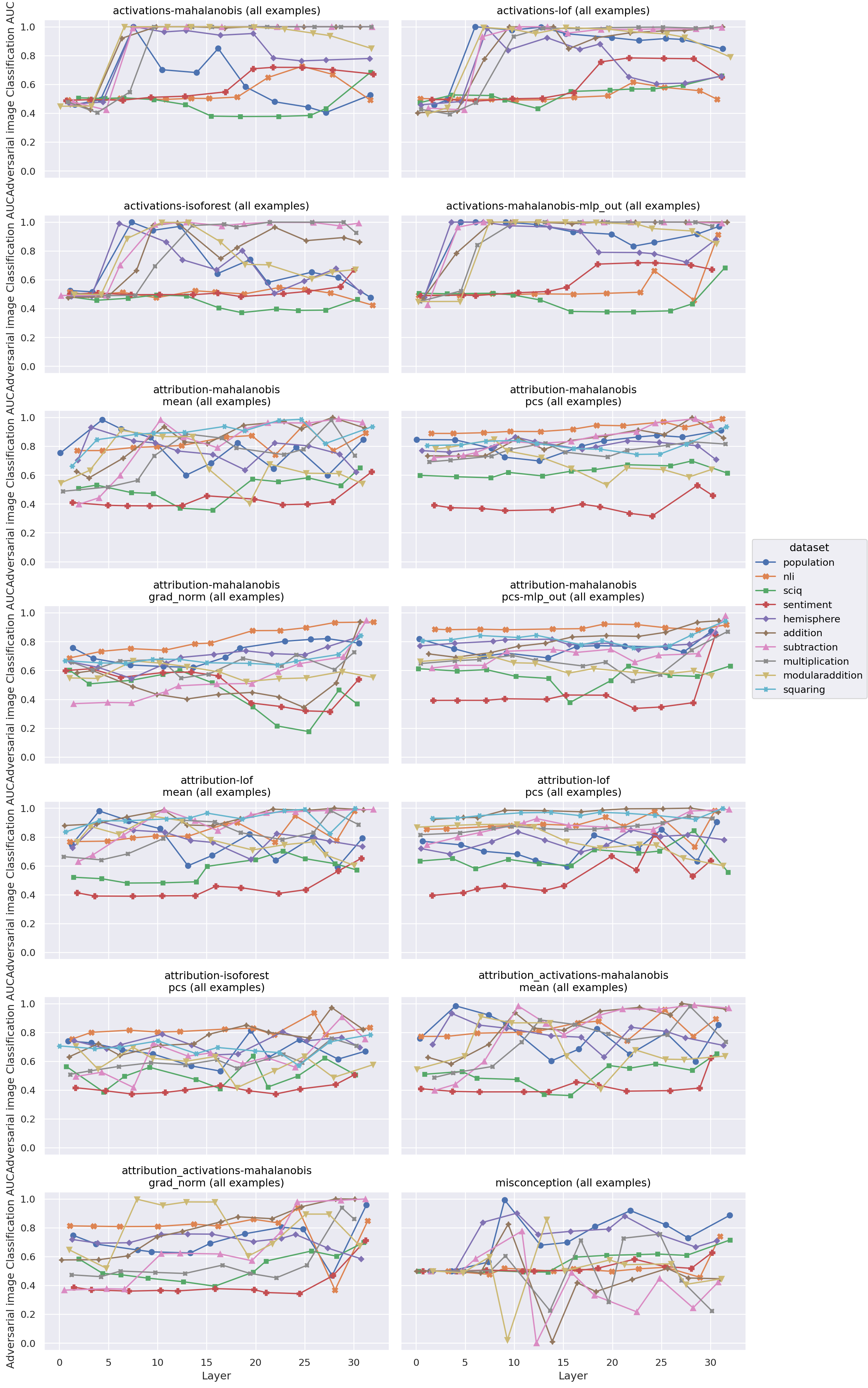Figure 3: Performance of different online detectors by layer

Offline detectors

Aggregated AUROC by offline score and features: all datasets

features	score	aggregated_mean_auc_roc	aggregated_mean_auc_roc_agree	aggregated_mean_auc_roc_disagree
activations	que	0.936	0.926	0.964
attribution	que concat mean	0.791	0.785	0.837
attribution	que grad norm	0.688	0.713	0.714
attribution	que pcs	0.840	0.837	0.856
probe	que concat mean	0.864	0.886	0.858
probe	que mean	0.860	0.878	0.854
probe	que pcs	0.860	0.866	0.872

Aggregated AUROC by offline score and features: by dataset

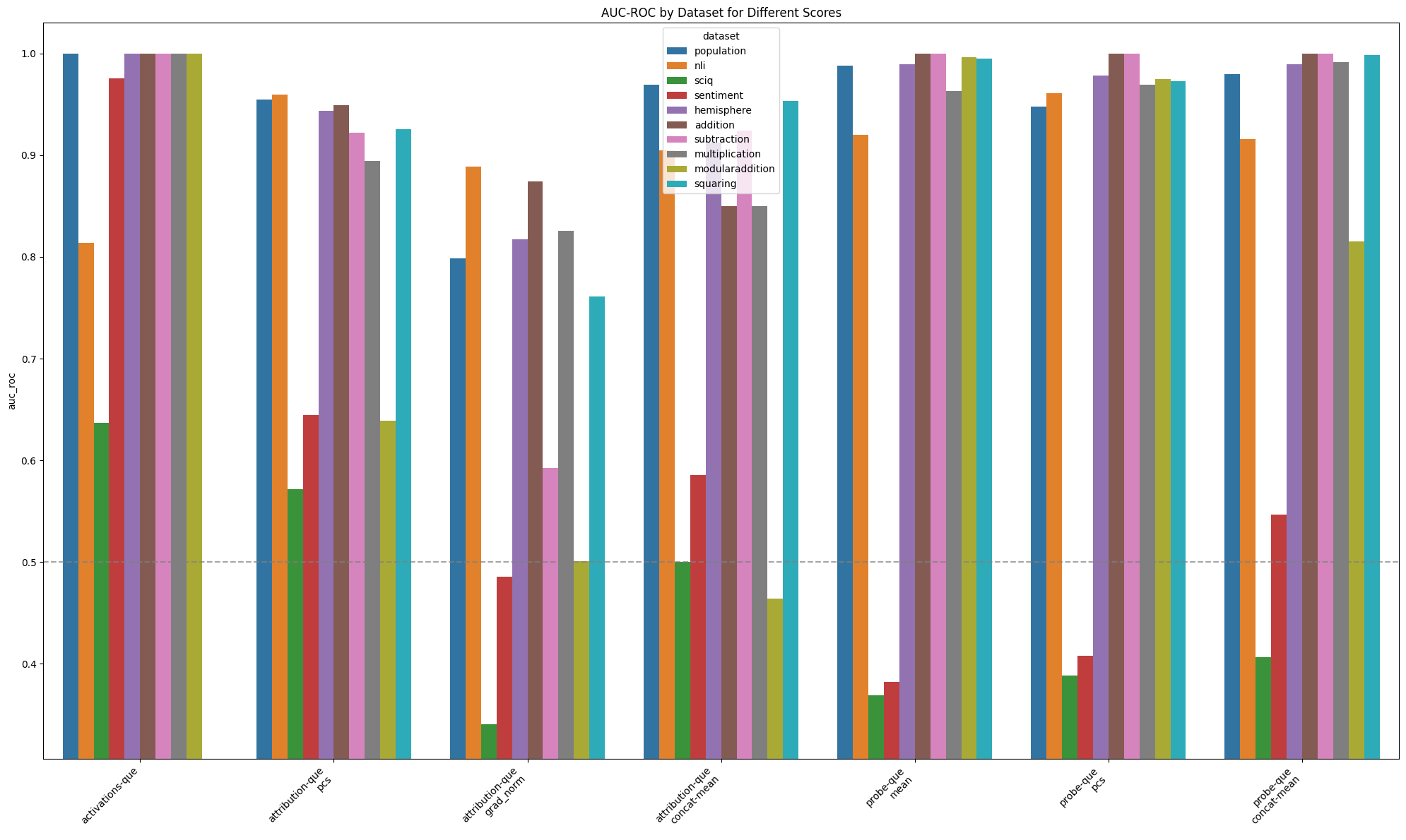Figure 4: Performance of different offline detectors where scores are aggregated across layers

Layerwise AUROC by offline score and features: by dataset

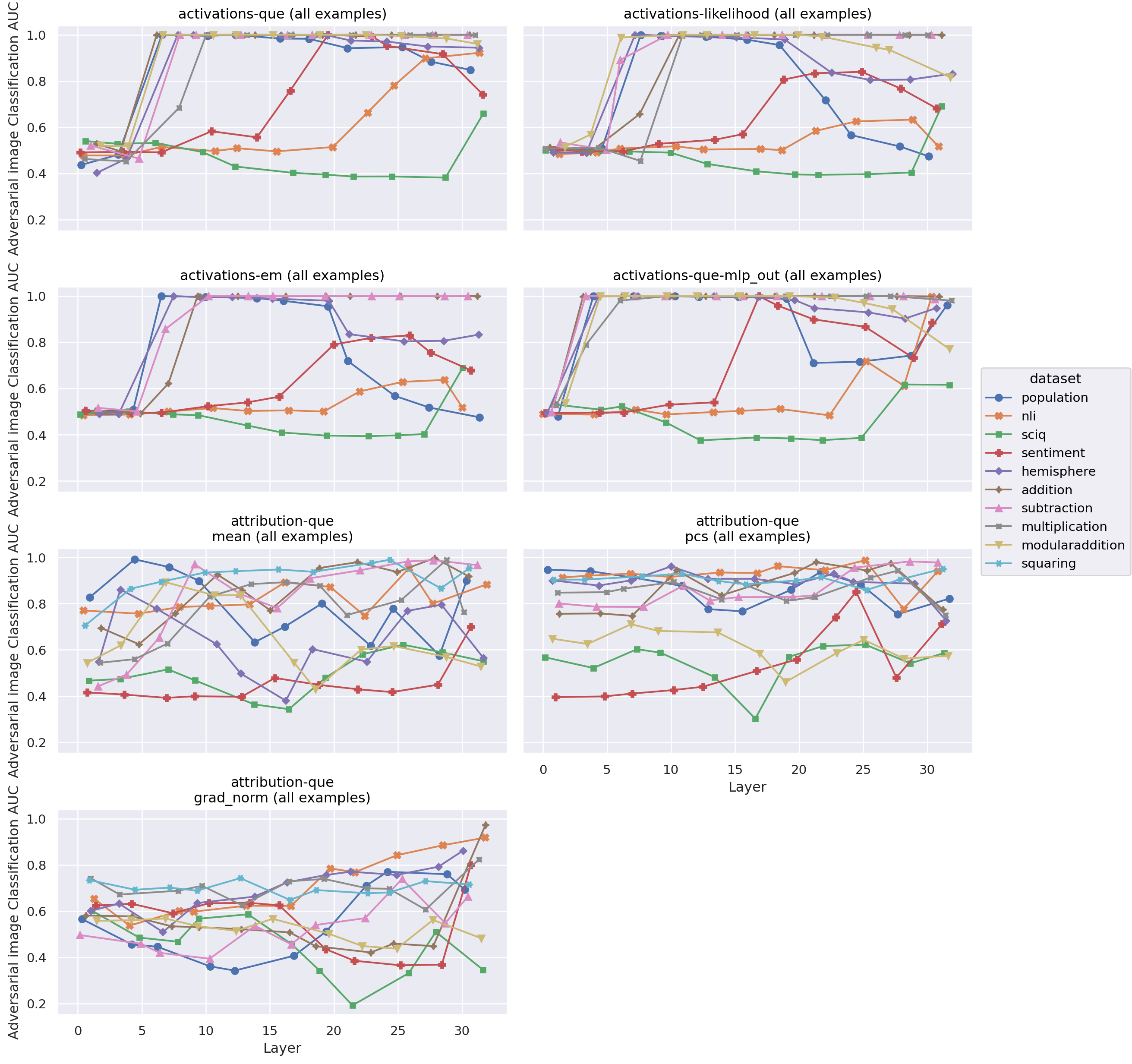Figure 5: Performance of different offline detectors by layer

Adversarial image detection

We conducted an exploratory experiment applying the same detectors to the task of detecting adversarial images for image classifiers. We focused on the Mahalanobis distance, because it worked well in comparison to other detectors for the quirky models task and because it is quite simple. We found that an activation-mahalanobis detector was able to detect adversarial images with an AUC of around 0.8 (layer-dependant) in a standard image classifier. It could not perform above chance for a robust classifier, however. Using attribution patching to approximate mean ablation along top principal components, on the other hand, had highly layer-dependent accuracy for a standard classifier. Interestingly, exactly the same approach performed marginally better than chance in a relatively layer independent manner for the tested robust detector. We did not test how robust the detectors themselves were to adversarial attack.

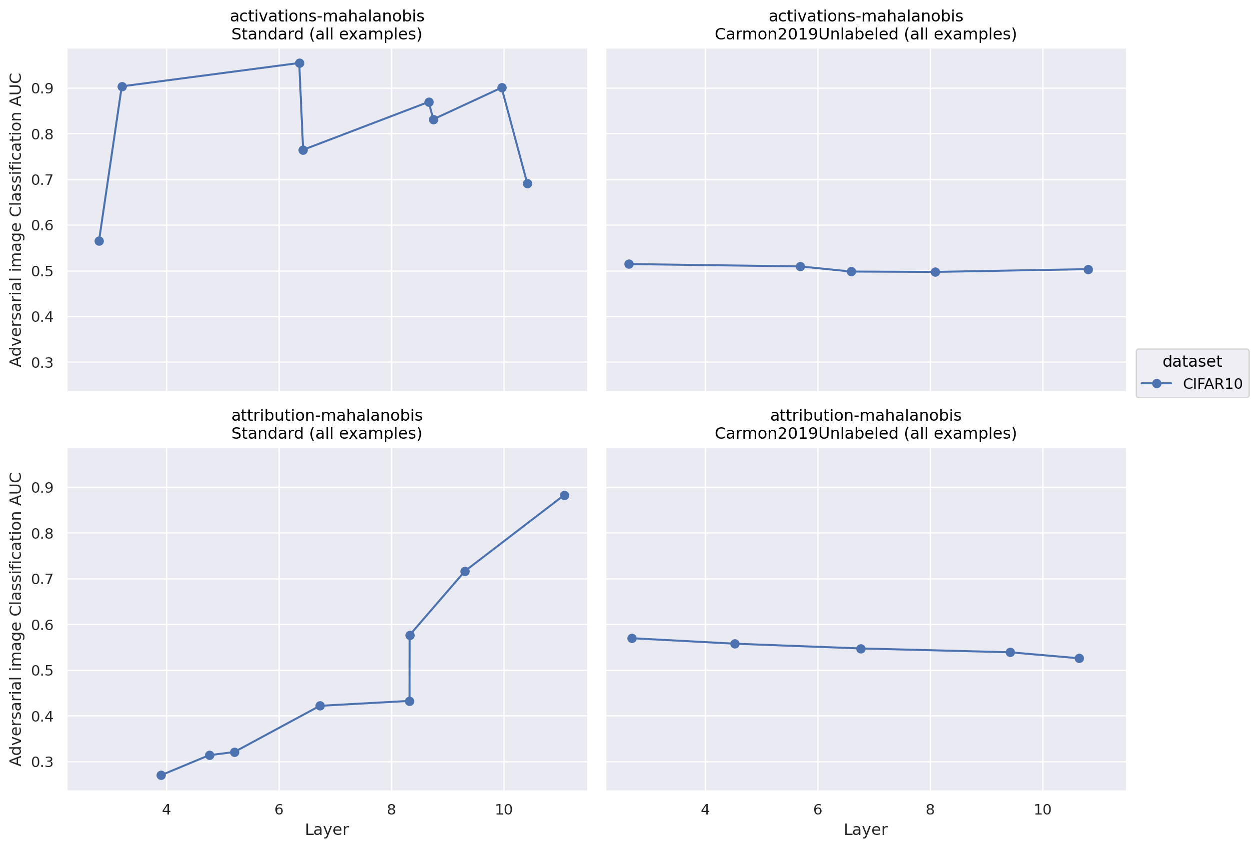Figure 6: Performance of different adversarial image detectors by layer and image model. Standard is a non-robust classifier, while Carmon2019Unlabeled is a robust model

Visualising features

In addition to testing various anomaly detectors, we also visualised per-layer activations and activation patching based effect estimates using UMAP and principal component plots. For "easy" dataset feature combinations (such as activations on the population dataset), we saw clear separation between normal and anomalous points among the top principal components in middle to late layers. We often (though not always) saw similar cluster separations in both principal component and UMAP plots.

Population

Activations

Layer 1

At layer 1, activations show a strong clustering pattern in both PCA and UMAP plots that does not correspond to any of the classes we have distinguished (true/false, trusted/test, normal/anomalous, agree/disagree).

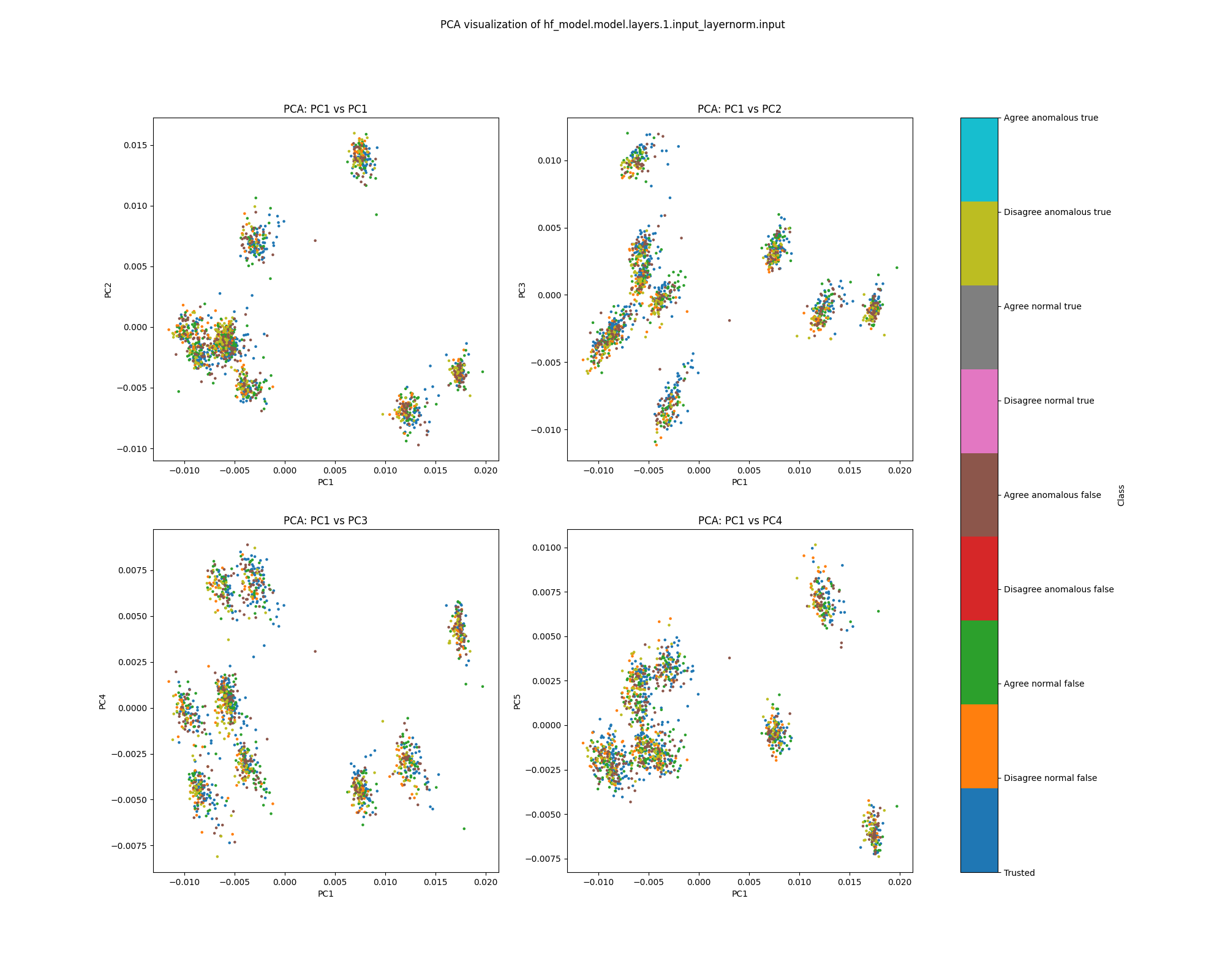Figure 7: PCA plot of population activations, layer 1

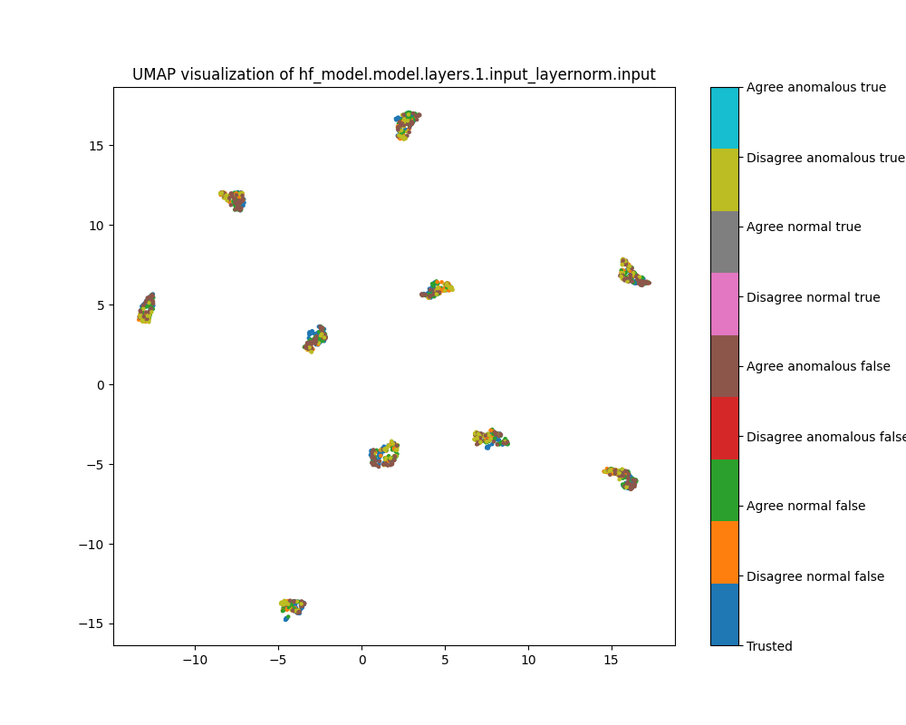Figure 8: UMAP plot of population activations, layer 1

Layer 16

In the layer 16 activations, the PCA plots show clear separation of anomalous and normal examples in the direction of the top principal component. In the direction of the second principal component, there is substantial separation between the trusted data used to train the detector and the normal test examples, showing that there is a distribution shift between the easy and hard examples. The population dataset consists of questions like input: "Does {character} think that {city} has a population greater than {population}?", and the difficulty metric is -log(population), so it is possible that the second principal component tracks log population.

While the PCA plots for layer 16 activations show different directions that seem to correspond to normal/anomalus, easy/hard and true/false, the UMAP plot separates all of these classes at once.

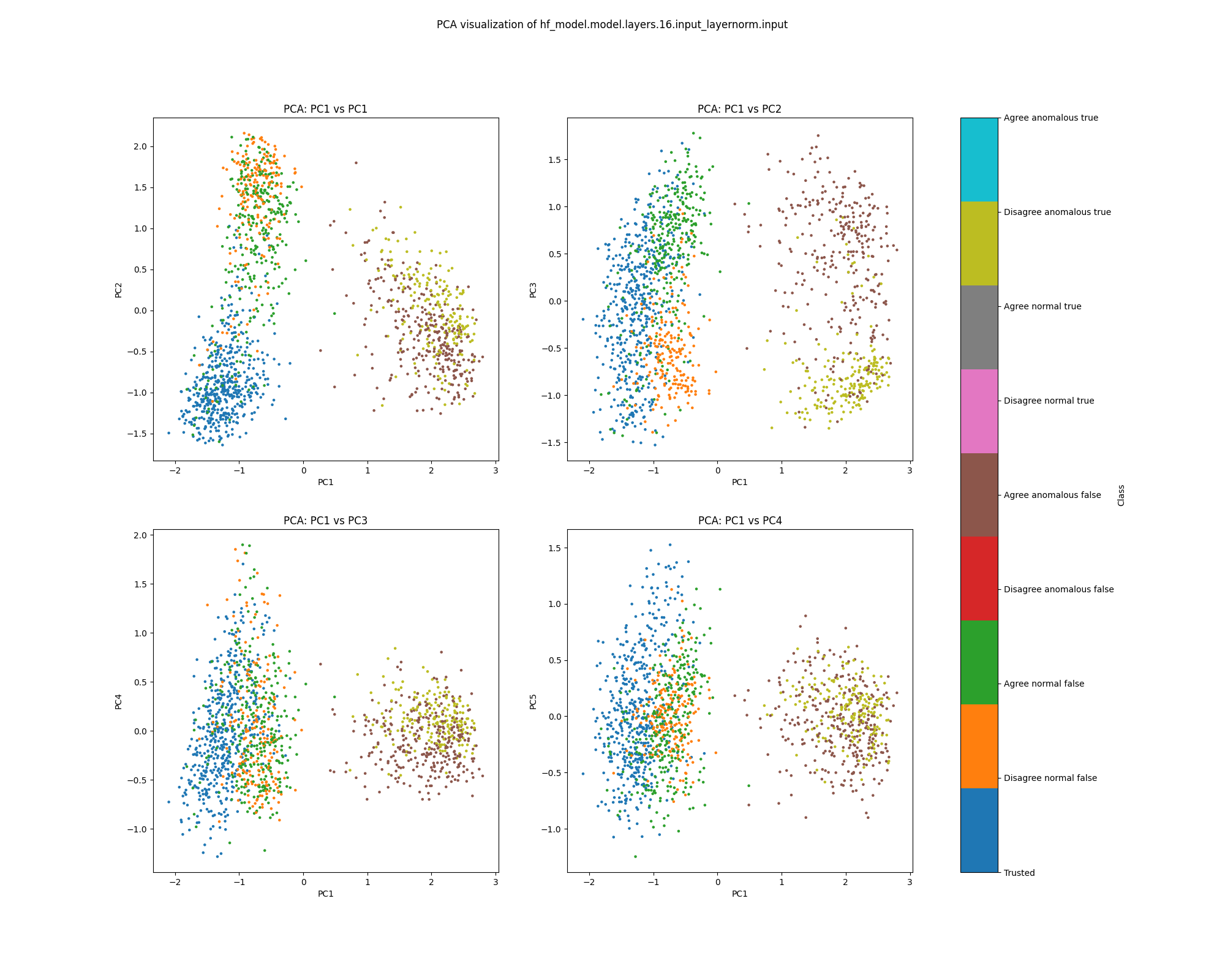Figure 9: PCA plot of population activations, layer 16

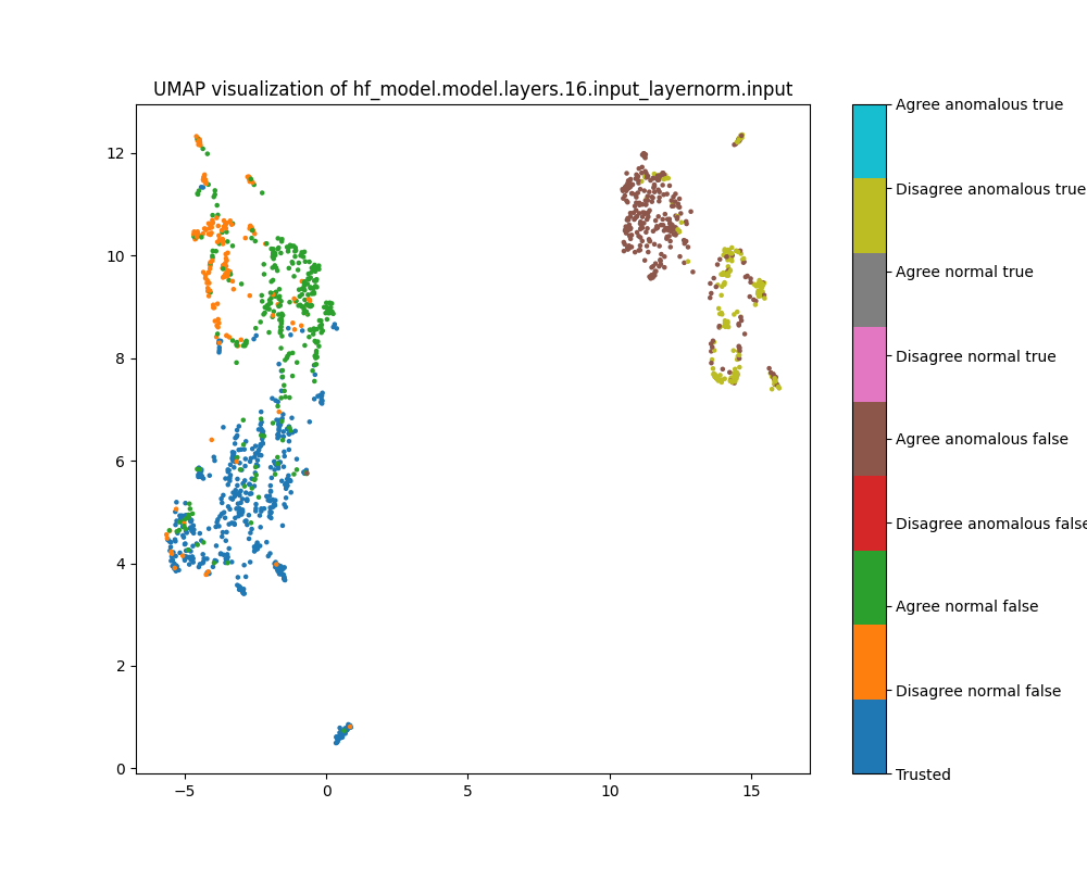Figure 10: UMAP plot of population activations, layer 16

Layer 28

By layer 28, clusters visible at layer 16 appear to have separated further. We also see the emergence of further structure that does not correspond to any of the classes we distinguish by colour.

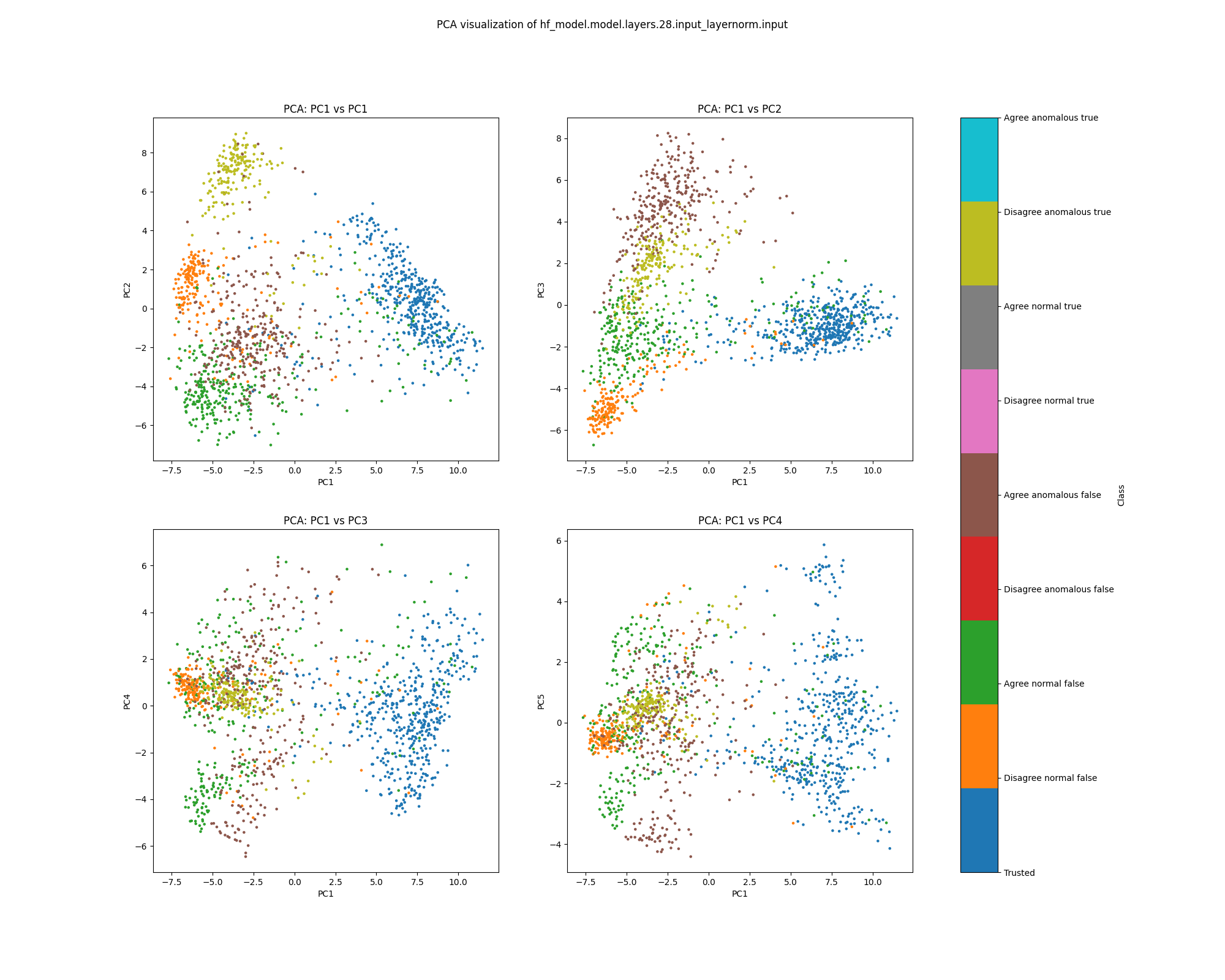Figure 11: PCA plot of population activations, layer 16

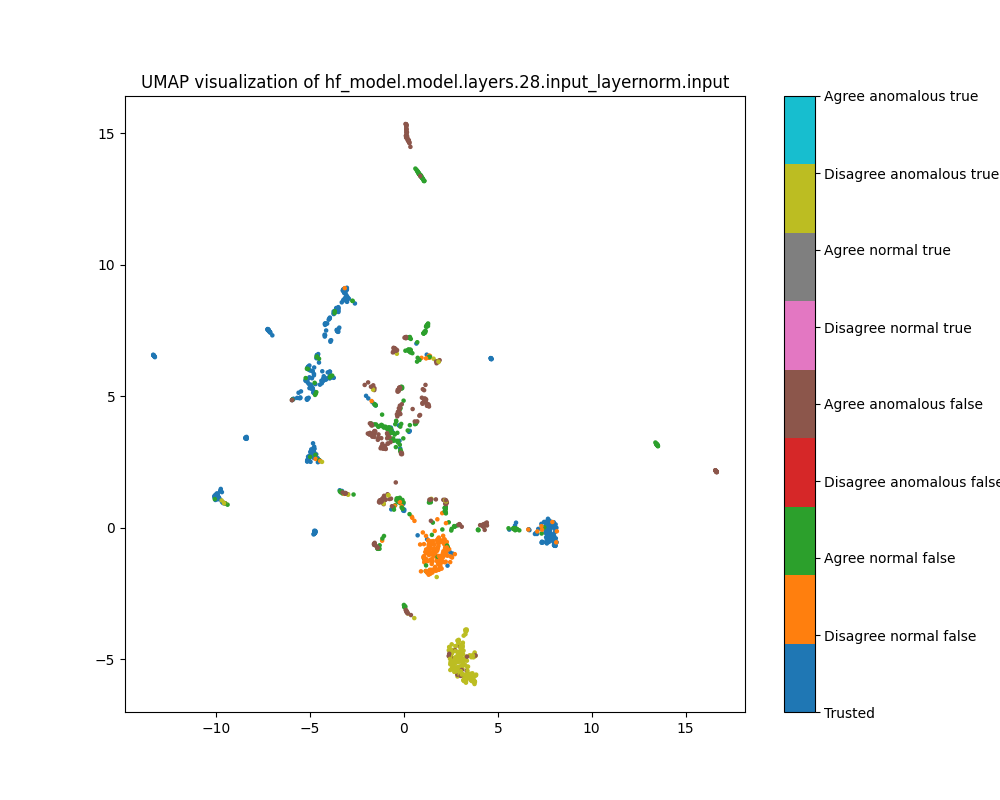Figure 12: UMAP plot of population activations, layer 16

Attention head mean ablations

Layer 1

For estimated mean ablation effects at layer 1, we see that anomalous examples are far more variable along the top principal component than normal examples, though they do not separate into different classes along any of the top principal components.

The UMAP plot, on the other hand, clearly distinguishes normal from anomalous examples. The anomalous examples have an interesting "double spike" shape. This might reflect the fact that interventions in the first layer might ablate the "Bob" label, and perhaps the spiky shapes reflect the sizes of the errors Bob made (we haven't checked this). Given this structure, it is surprising that the local outlier factor score with attribution based features does not perform better for the population dataset in layer 1, given that both local outlier factor and UMAP depend on the neighbourhoods of points.

Figure 13: PCA plot of population mean ablations, layer 1

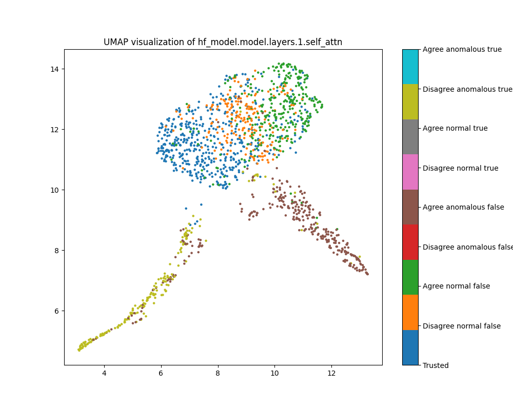Figure 14: UMAP plot of population mean ablations, layer 1

Layer 16

While clustering by the classes we have coloured is evident in layer 16 mean ablation effect estimates, it is far less defined than the clustering evident in layer 16 activations.

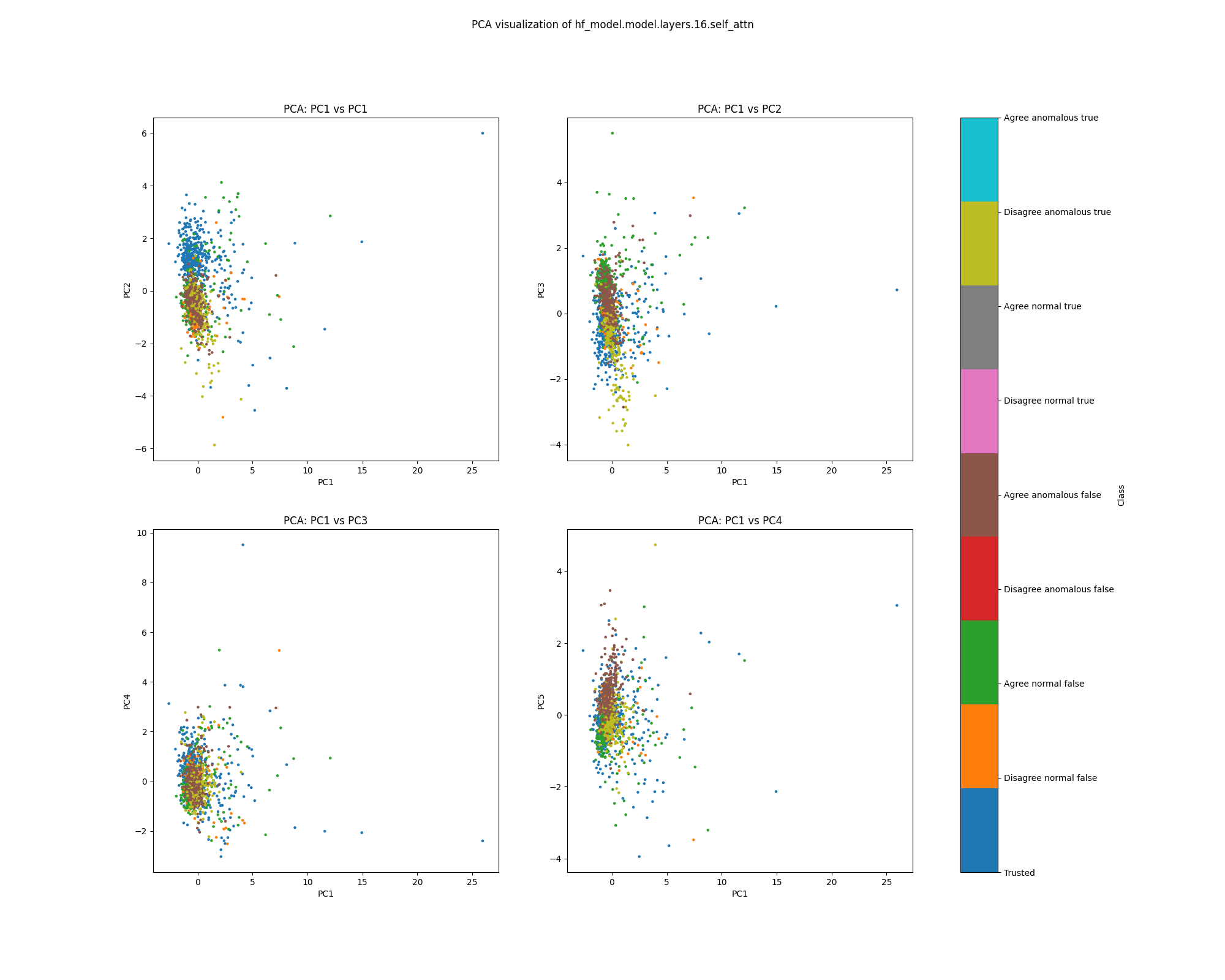Figure 15: PCA plot of population mean ablations, layer 1

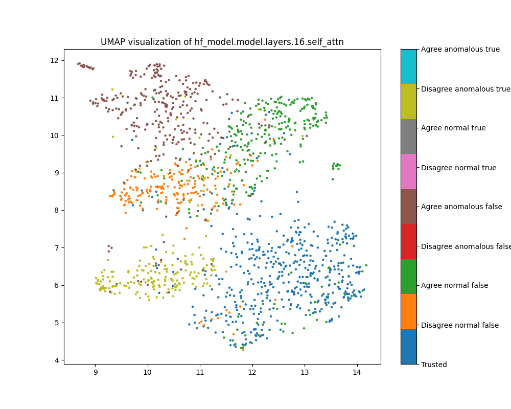Figure 16: UMAP plot of population mean ablations, layer 1

Layer 28

By layer 28, clusters visible at layer 16 appear to have separated further. We also see the emergence of further structure that does not correspond to any of the classes we distinguish by colour.

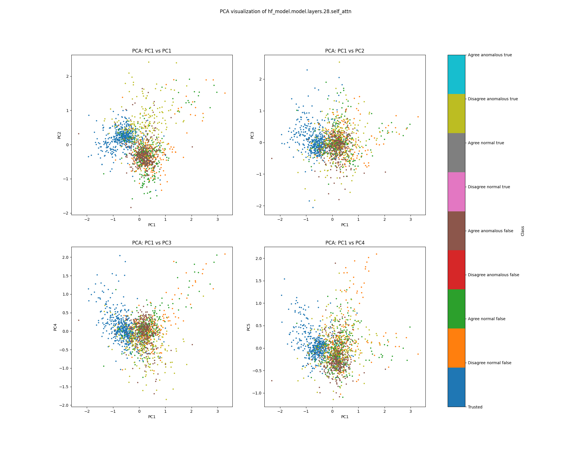Figure 17: PCA plot of population activations, layer 28

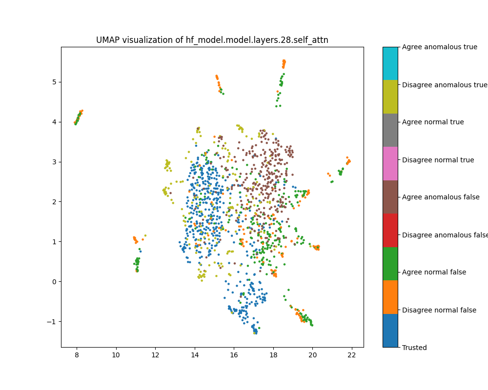Figure 18: UMAP plot of population activations, layer 28

Probe shift

The probe shift method preserves the structure visible in layer 4 of the mean ablation UMAP plot throughout every layer of the network. This may be attributable to the possibility that there is an intervention in layer 1 that ablates the "Bob" label, and this has a significant effect on the accuracy of probes throughout the network.

Layer 4

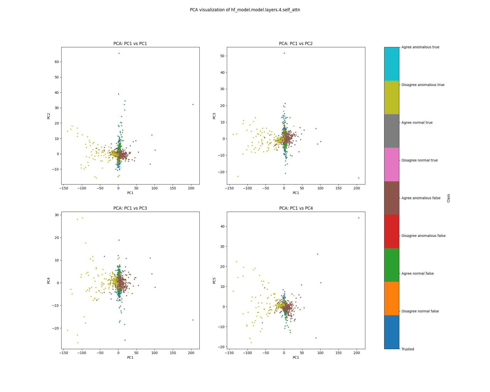Figure 19: PCA plot of population probe shift features, layer 4

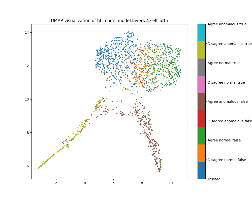Figure 20: UMAP plot of population probe shift features, layer 4

Layer 16

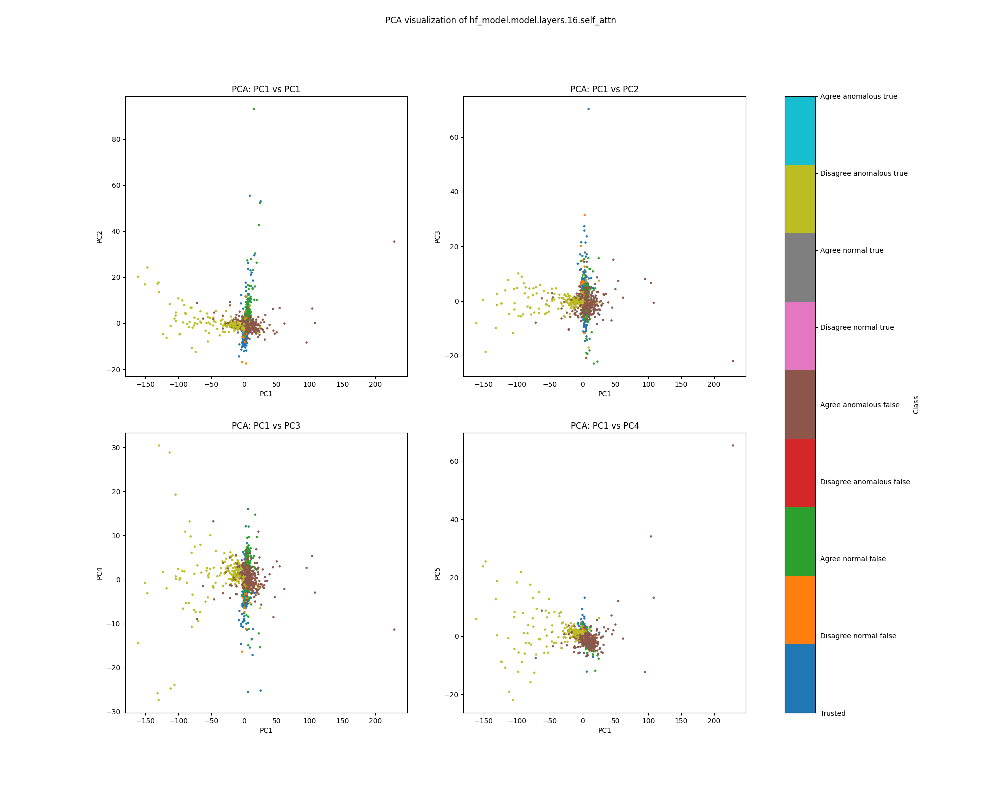Figure 21: PCA plot of population probe shift features, layer 16

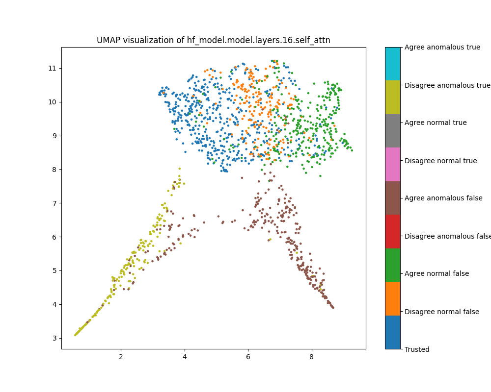Figure 22: UMAP plot of population probe shift features, layer 16

Layer 28

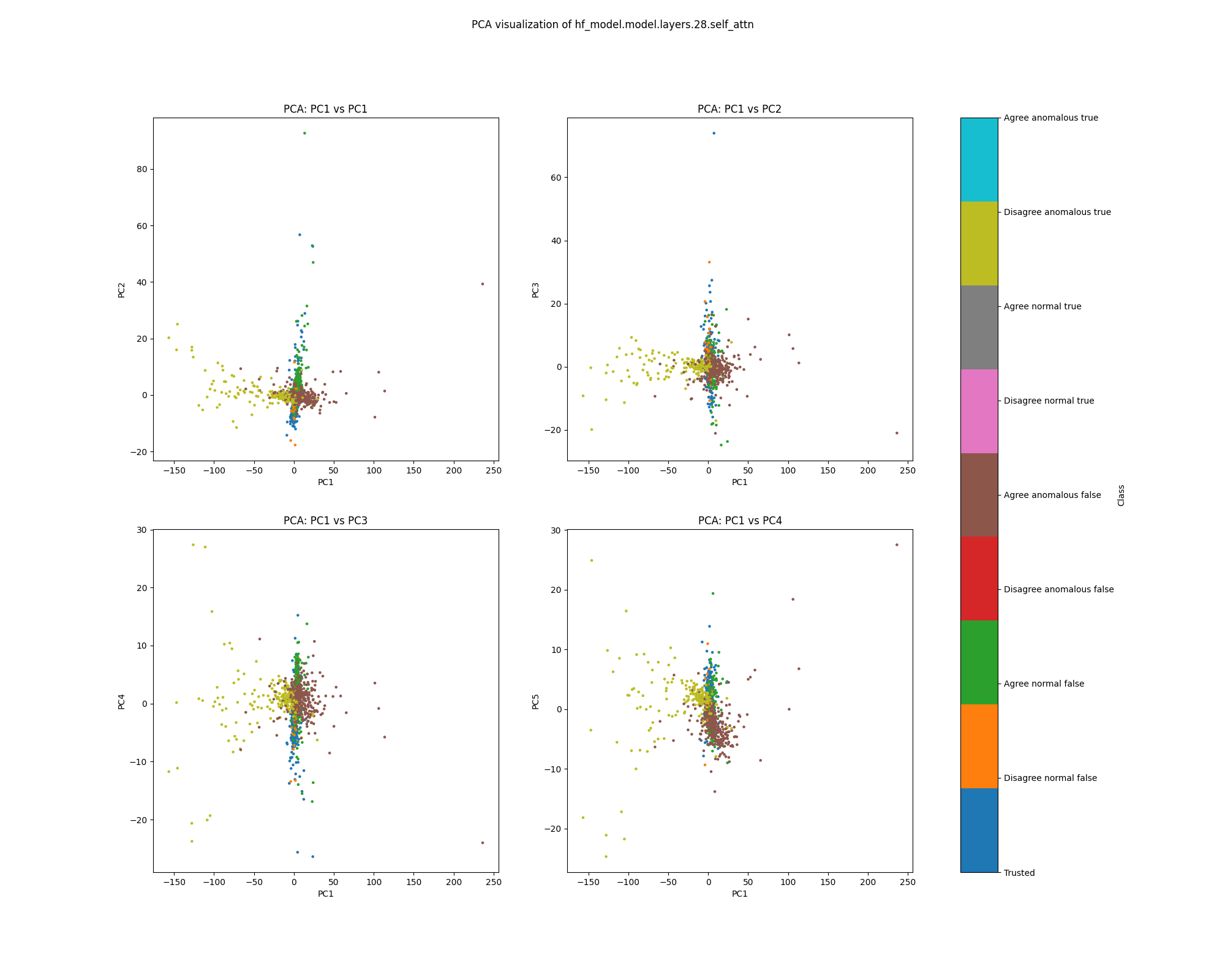Figure 23: PCA plot of population probe shift features, layer 28

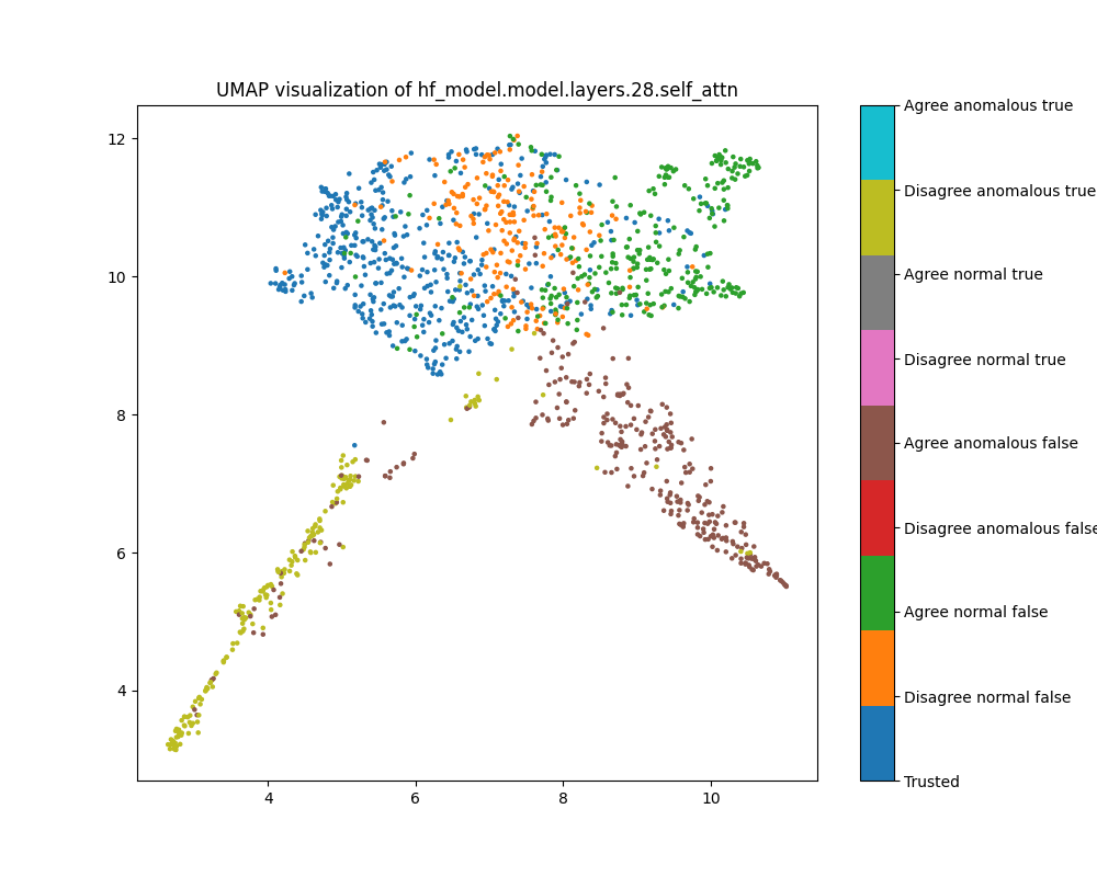Figure 24: UMAP plot of population probe shift features, layer 28

Sentiment

While population is a relatively easy dataset, sentiment is more challenging. Attribution based methods performed worse than change on it, while activation based detectors could not reliably distinguish normal from anomalous examples.

Activations

Layer 1

Like the activations for population, layer 1 activations for sentiment form clusters unrelated to our labelling. We do not see much separation between trusted and test examples.

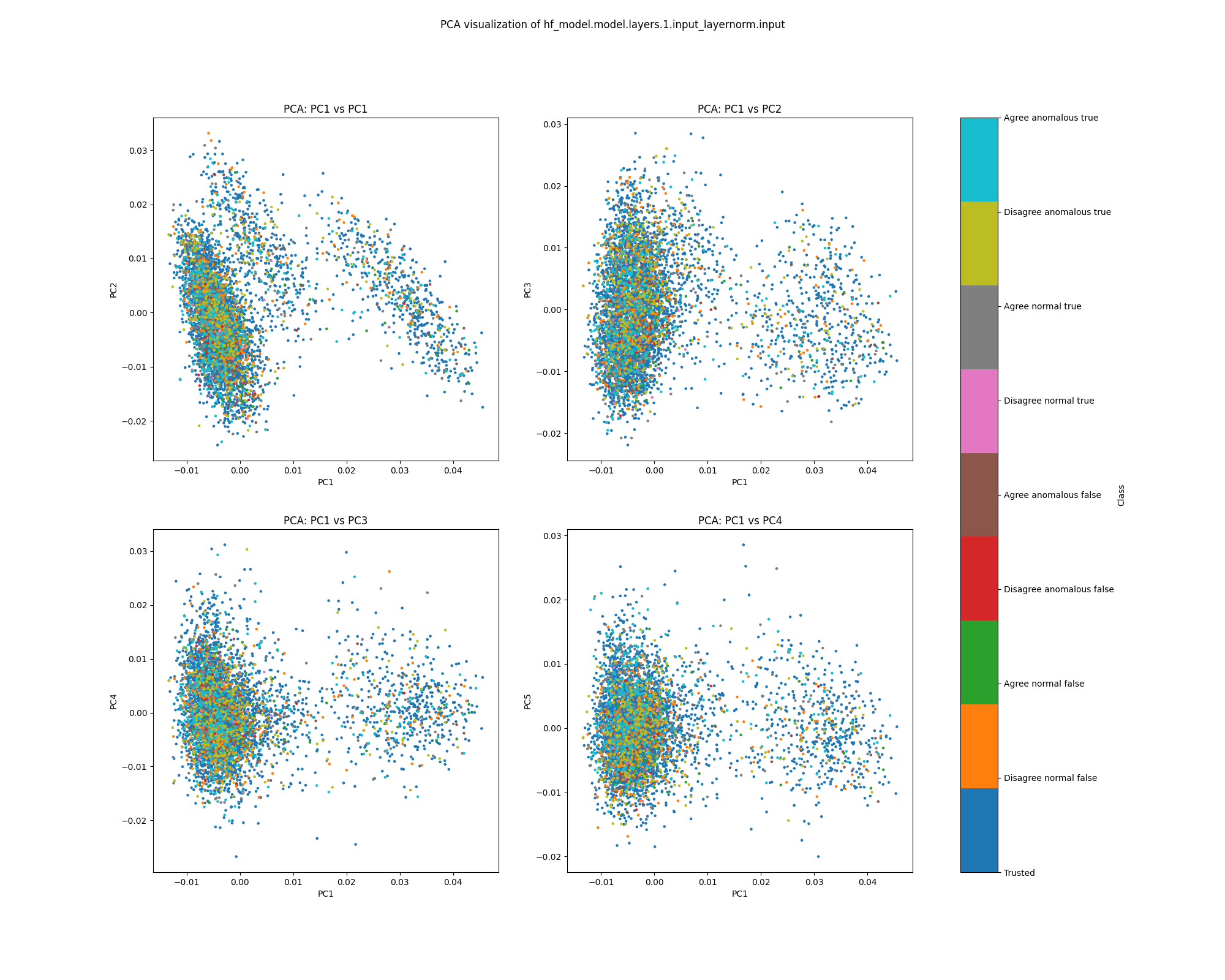Figure 25: PCA plot of activations for sentiment, layer 1

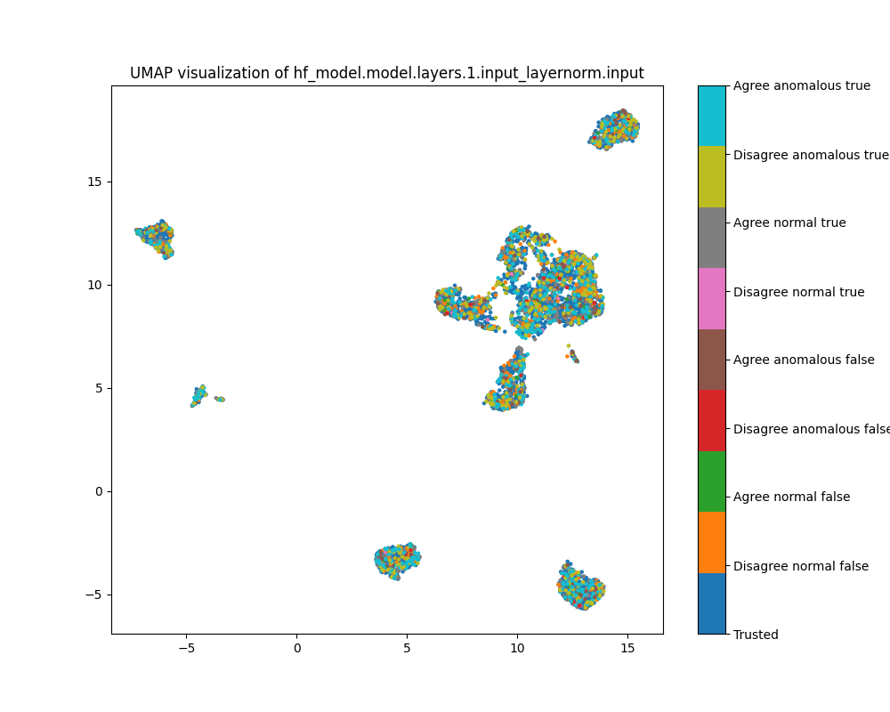Figure 26: UMAP plot of activations for sentiment, layer 1

Layer 16

At layer 16, we see separation between true and false examples, as well as imperfect separation between examples where Alice and Bob agree and where Alice and Bob disagree. We do not see separation in either PCA or UMAP plots between normal and anomalous examples, nor between trusted and test examples.

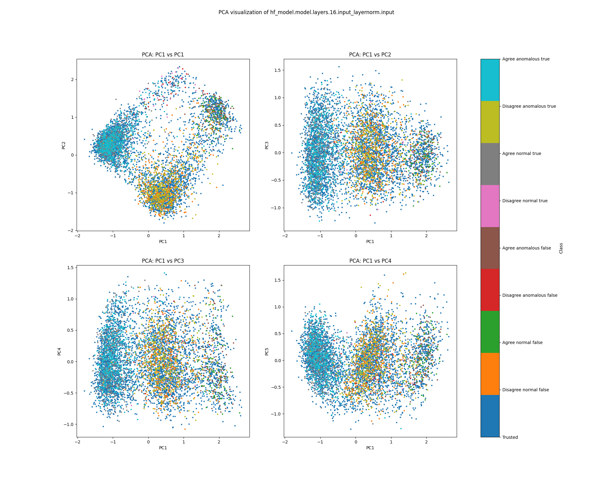Figure 27: PCA plot of activations for sentiment, layer 16

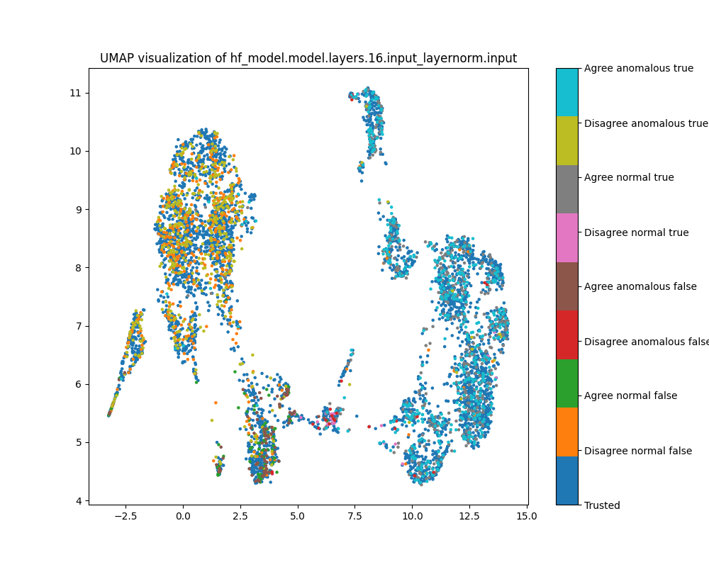Figure 28: UMAP plot of activations for sentiment, layer 16

Layer 28

By layer 28, we see a little separation between normal and anomalous examples, particularly examples where Alice and Bob agree and the label is true. We see further separation between true and false examples, as well as between examples where Alice and Bob agree and disagree.

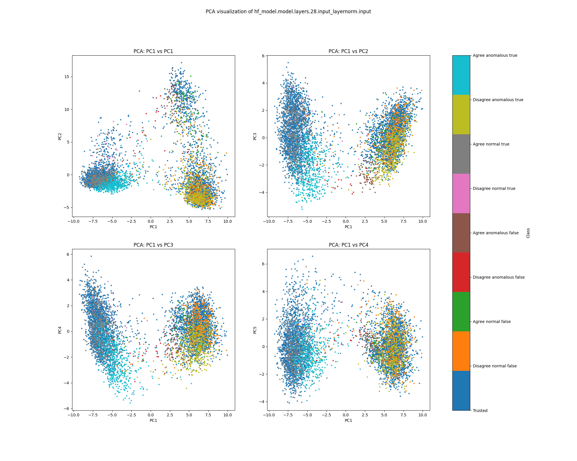Figure 29: PCA plot of activations for sentiment, layer 28

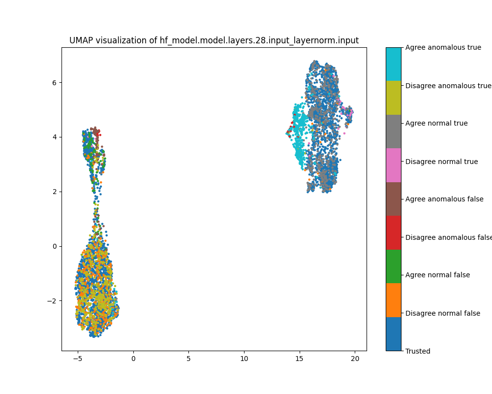Figure 30: UMAP plot of activations for sentiment, layer 28

Attention head mean ablations

Layer 1

For early to mid layer PCA plots of attention head mean ablations, we see little structure, though we can see disagree anomalous true examples distinguished from others in the direction of PC1. In UMAP plots, we see the familiar distinction between true and false and agree and disagree examples, though without visible clustering.

Figure 31: PCA plot of attention head mean ablations for sentiment, layer 1

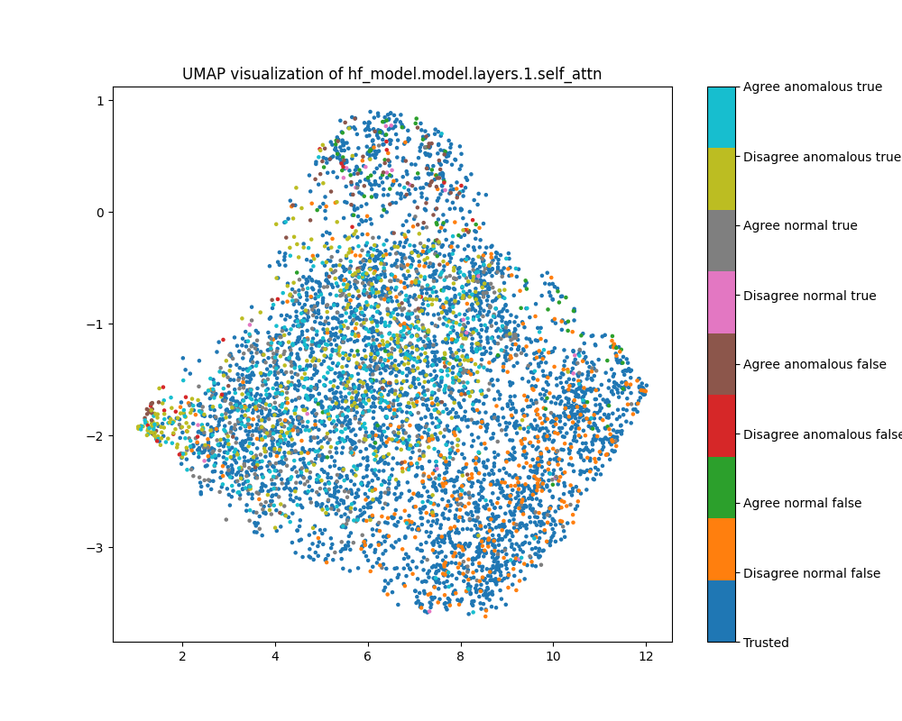Figure 32: UMAP plot of attention head mean ablations for sentiment, layer 1

Layer 16

Our remarks for layer 1 remain largely applicable to layer 16.

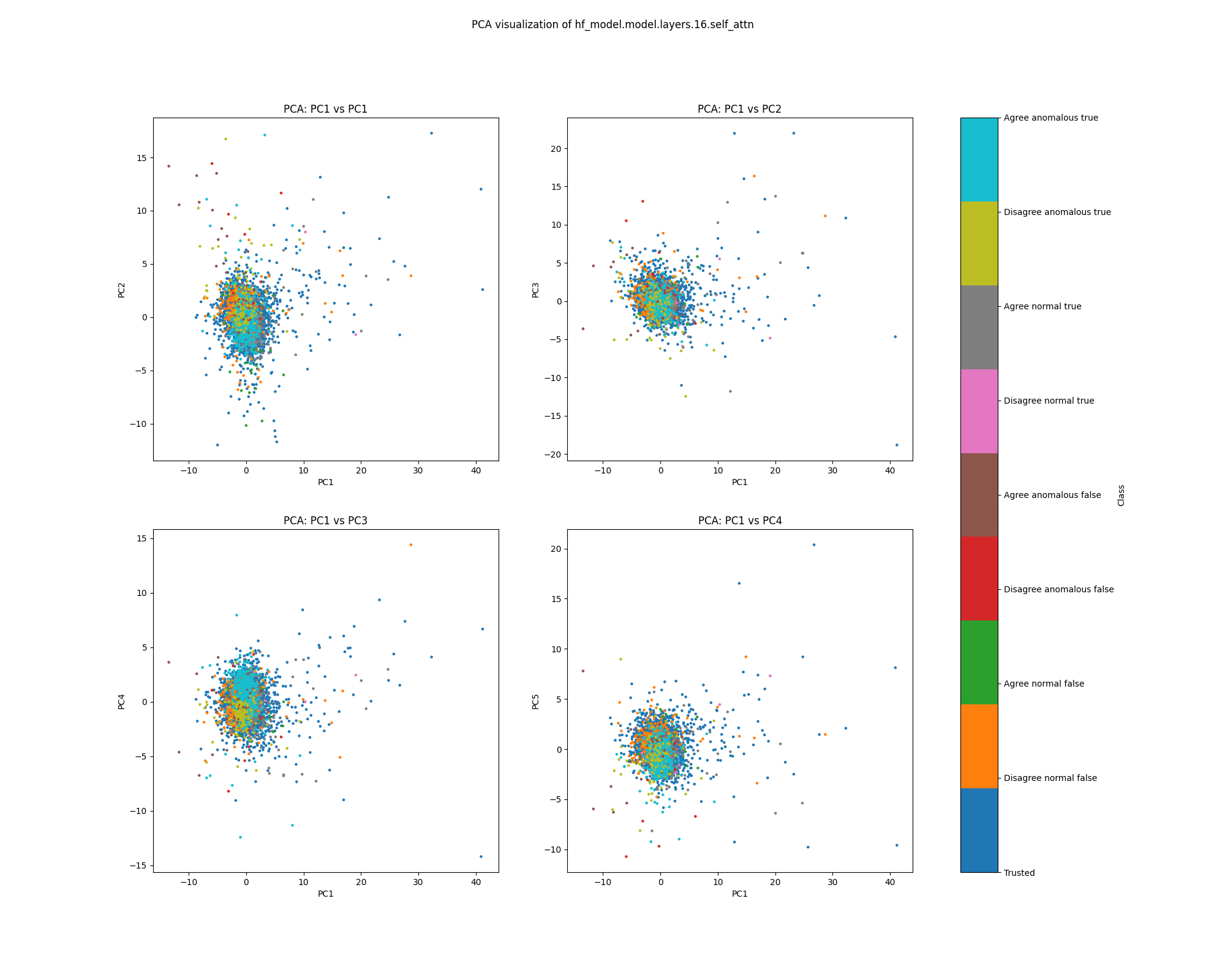Figure 33: PCA plot of attention head mean ablations for sentiment, layer 16

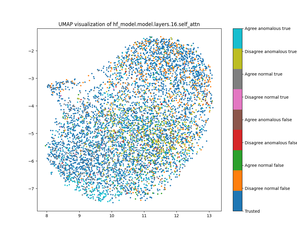Figure 34: UMAP plot of attention head mean ablations, layer 16

Layer 28

In layer 28 we see some separation of normal from anomalous examples, particularly in the UMAP plot. This corresponds to our observation that later layers were associated with better scores for the attribution-LOF detector.

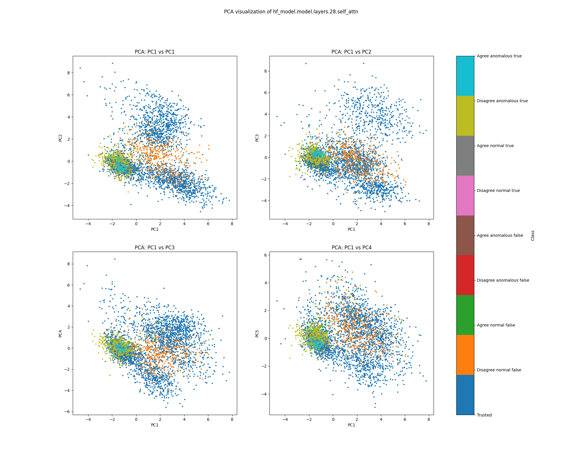Figure 35: PCA plot of attention head mean ablations for sentiment, layer 28

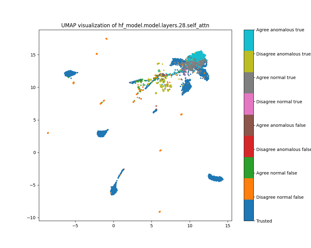Figure 36: UMAP plot of attention head mean ablations for sentiment, layer 28

Probe shift

Layer 4

Like attention head mean ablation, probe shift features show separation between true and false and agree and disagree, but generally not separation from trusted data overall, though there is a small cluster of anomalous data that is separated from the trusted data present in all layers.

In the UMAP visualisation, anomalous examples are strongly clustered and separated from

Figure 37: PCA plot of probe shift features for sentiment, layer 4

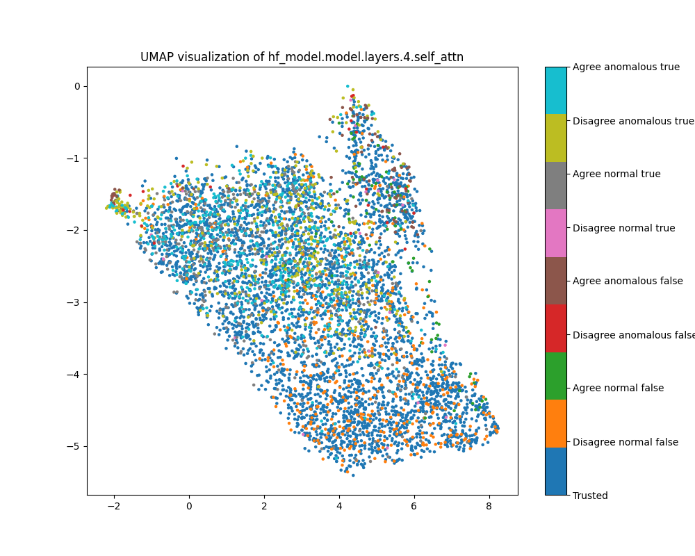Figure 38: UMAP plot of probe shift features for sentiment, layer 4

Layer 16

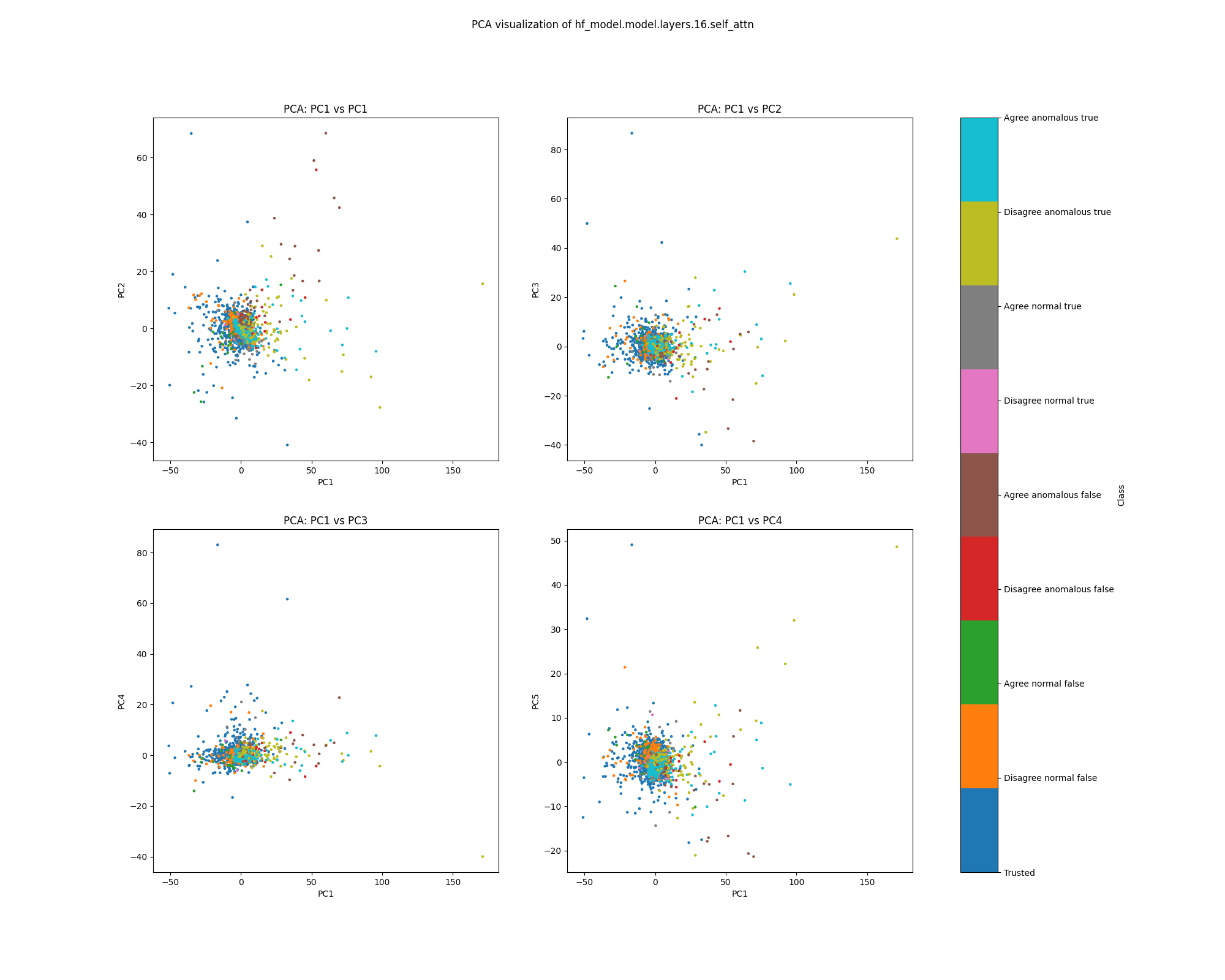Figure 39: PCA plot of probe shift features for sentiment, layer 16

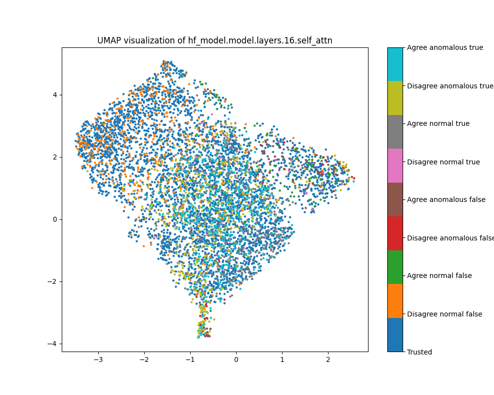Figure 40: UMAP plot of probe shift features for sentiment, layer 16

Layer 28

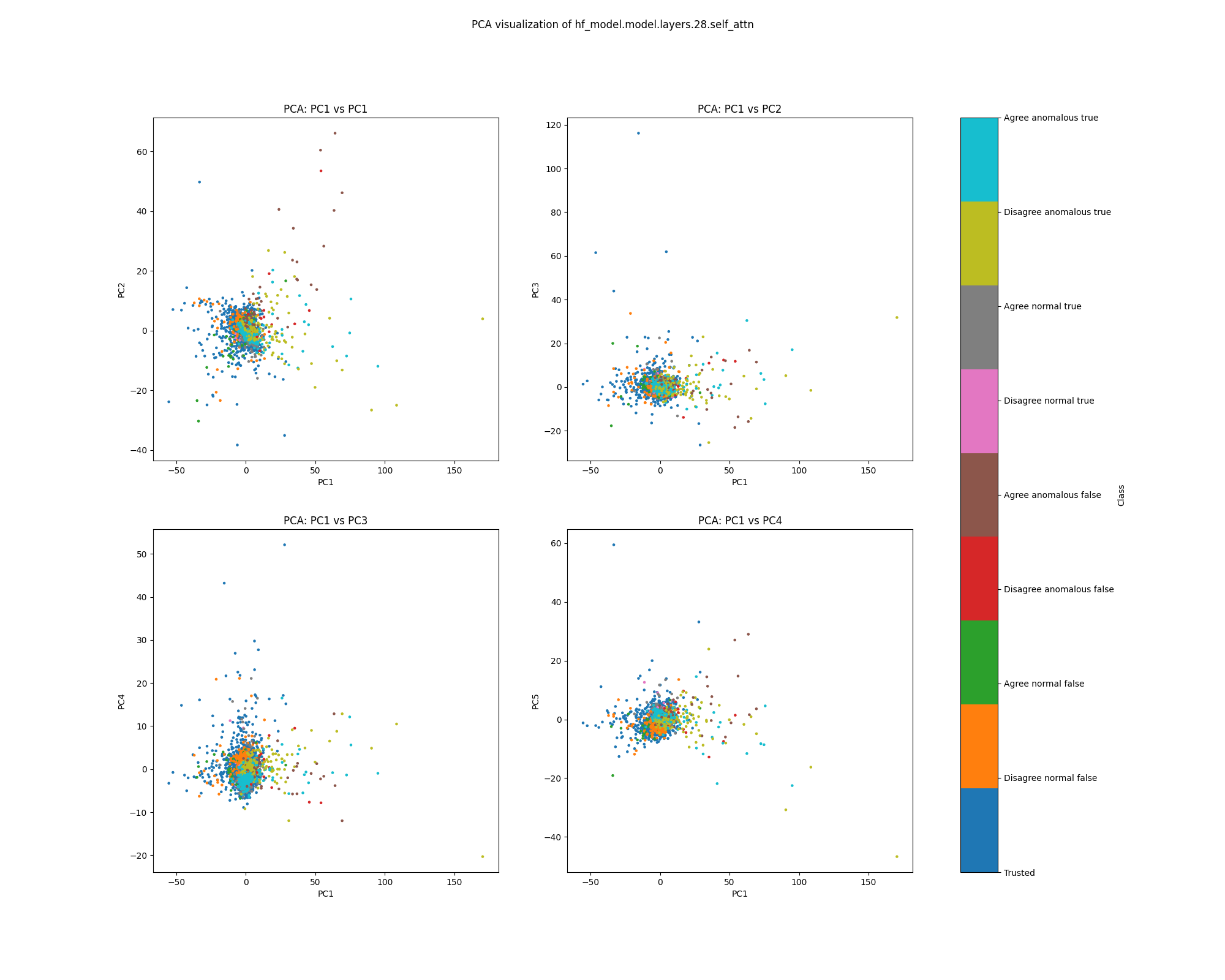Figure 41: PCA plot of probe shift features for sentiment, layer 28

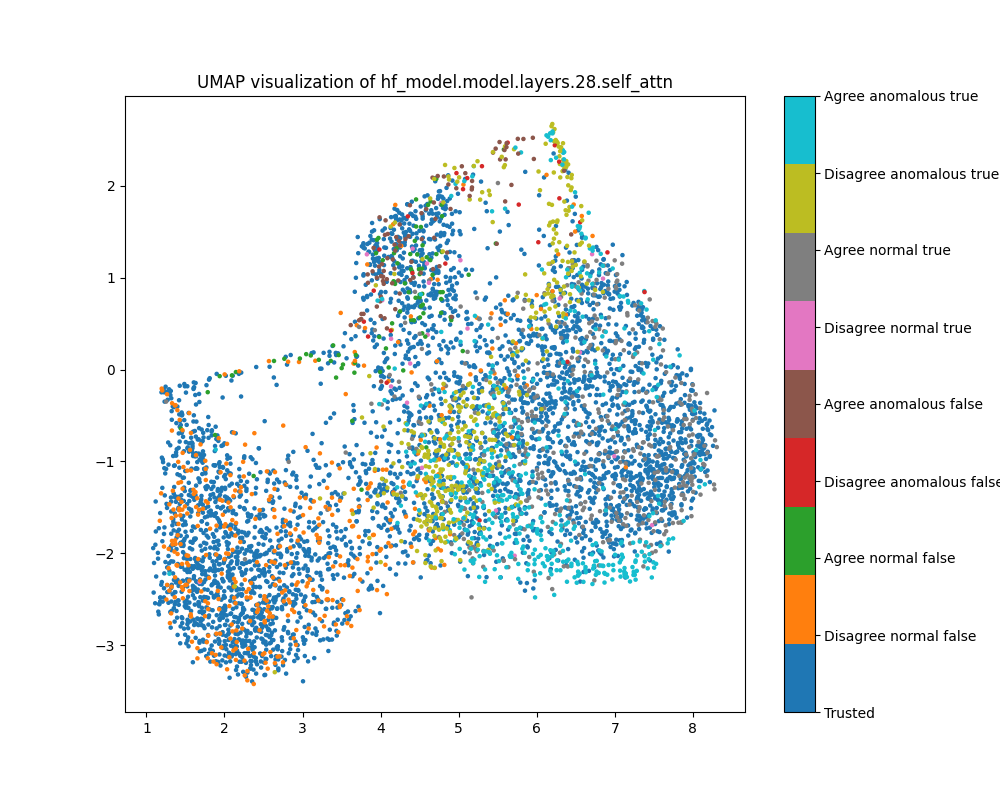Figure 42: UMAP plot of probe shift features for sentiment, layer 28

Discovering functional elements of the network with edge attribution patching

We also experimented with edge attribution patching, a method of automated circuit discovery. In comparison with mean ablation of attention heads, this approach

• Used "edge patching" for a finer grained set of effects to study
• Examined interventions on MLPs as well as attention heads
• Patched activations from each "Alice" prompt with those from an identical "Bob" prompt

Edge patching computes the effects of replacing the activations at the output of some unit (e.g. an attention head or MLP layer) mediated by a downstream unit. That is, the approximate effect of intervening on an edge from unit A to unit B on a score $S$ is given by

$$\Delta S = (o_A - o_A')^T \frac{\partial S}{\partial i_B}$$

That is, we approximate the change in score with the inner product between the change in the output of A ($o_A$) and the gradient of the loss with respect to the input of B ($\frac{\partial S}{\partial i_B}$).

Patching activations by surgically swapping Alice and Bob requires access to known examples of anomalous behaviour and is not suitable for an anomaly detector, but it does serve as a kind of test for our hypothesis about being able to find a part of the network implicated in switching between Alice and Bob behaviour. In fact, from testing on a few datasets, we find an edge from MLP 30 to MLP 31 that appears to play a large role in behaviour switching for multiple datasets (Figure 5). Because this edge is between two MLP layers, we could not have discovered it using attention head patching.

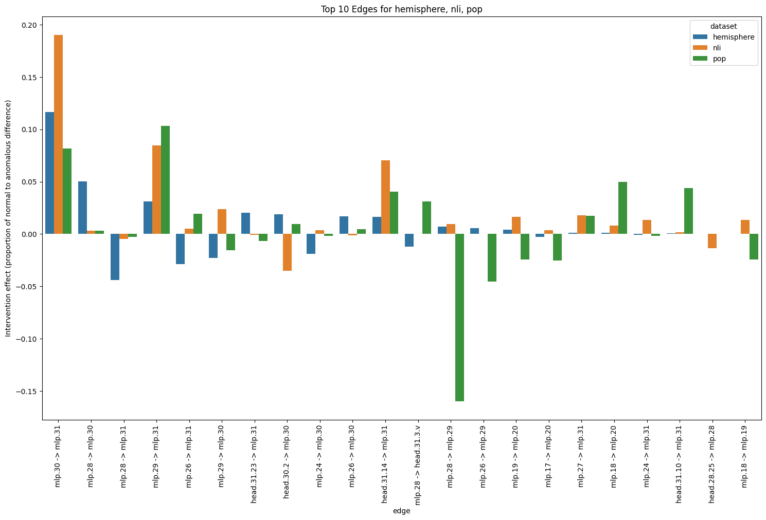Figure 43: Top 10 edges for nli, population and hemisphere datasets

We are planning to experiment with sparse autoencoders

We have mentioned that one of the key challenges is finding a good activation or effect basis to compute anomaly scores. We have experimented with the eigenbasis of the covariance matrices of the activations in each layer, and are looking to try "edge interventions" as defined in the previous section. We have no strong reason to expect either of these is a great basis for anomaly detection.

Sparse autoencoders (SAEs) are another approach to defining a basis for investigating model behaviour. A sparse autoencoder learns a sparse codebook of features which can be used to reconstruct the activations. Given an example, we expect the active features in the codebook are the most important features for explaining the model's behaviour. It is plausible that Alice and Bob behaviour is distinguished by differing distributions of codebook features, corresponding to different concepts invoked by the different modes of operation. Alternatively, perhaps the model computes both Alice and Bob answers for each prompt and then chooses one at the end. In this case, we may or may not see different feature activations, but we would expect to see different effects of intervening on Alice features if the prompt contains "Alice" or "Bob".

Outlook

We have strong MAD results for many datasets, but we would ideally like AUCs uniformly very close to 1 which we have not achieved. For some datasets (NLI, sentiment and sciq), model performance appears weaker and layer dependent even for the strongest MAD approaches. We have not yet found a compelling way to use attribution patching to improve our results. We are looking to experiment with sparse autoencoders for MAD soon, as we think it is plausible MAD in a basis where features are disentangled may be easier.

Appendix: Tables of Results

For reference, here are detailed AUROC scores for a large collection of detectors for each dataset. The "best" layer is chosen as the layer that maximises the average AUROC across all datasets.

Online methods

Addition results: online methods

score	features	mean_auc_roc	aggregated_auc_roc	best_auc_roc	mean_auc_roc_agree	aggregated_auc_roc_agree	best_auc_roc_agree	mean_auc_roc_disagree	aggregated_auc_roc_disagree	best_auc_roc_disagree	best_layer
	iterative rephrase	0.544	0.544	0.544	0.356	0.356	0.356	0.524	0.524	0.524	aggregate
	misconception contrast	0.447	0.408	0.408	0.445	0.401	0.401	0.437	0.383	0.383	aggregate
isoforest	activations	0.796	nan	0.996	0.792	nan	0.995	0.803	nan	0.997	13
isoforest mean	attribution	0.866	0.866	0.866	0.995	0.995	0.995	0.942	0.942	0.942	aggregate
isoforest pcs	attribution	0.765	nan	0.972	0.851	nan	0.999	0.874	nan	0.984	28
lof	activations	0.855	0.999	0.999	0.853	0.999	0.999	0.857	0.999	0.999	aggregate
lof concat mean	probe	0.999	0.999	0.999	0.997	0.997	0.997	1.000	1.000	1.000	aggregate
lof concat pcs	probe	1.000	1.000	1.000	1.000	1.000	1.000	1.000	1.000	1.000	aggregate
lof mean	attribution	0.946	0.997	0.997	0.977	1.000	1.000	0.979	1.000	1.000	aggregate
lof mean	probe	0.947	1.000	1.000	0.947	1.000	1.000	0.965	1.000	1.000	aggregate
lof pcs	attribution	0.974	0.995	0.997	0.987	1.000	0.999	0.998	1.000	1.000	25
lof pcs	probe	0.930	nan	1.000	0.946	nan	1.000	0.962	nan	1.000	28
mahalanobis	activations	0.900	1.000	1.000	0.898	1.000	1.000	0.902	1.000	1.000	aggregate
mahalanobis concat mean	attribution	0.853	0.853	0.853	0.950	0.950	0.950	0.992	0.992	0.992	aggregate
mahalanobis concat mean	probe	1.000	1.000	1.000	1.000	1.000	1.000	1.000	1.000	1.000	aggregate
mahalanobis grad norm	attribution	0.509	nan	0.939	0.410	nan	0.980	0.652	nan	0.944	31
mahalanobis grad norm	attribution activations	0.799	nan	0.999	0.871	nan	1.000	0.853	nan	1.000	31
mahalanobis mean	attribution	0.856	0.993	0.993	0.898	1.000	1.000	0.923	1.000	1.000	aggregate
mahalanobis mean	attribution activations	0.859	1.000	1.000	0.899	1.000	1.000	0.923	1.000	1.000	aggregate
mahalanobis mean	probe	0.940	1.000	1.000	0.943	1.000	1.000	0.952	1.000	1.000	28
mahalanobis mean	probe activations	0.243	nan	0.488	0.243	nan	0.493	0.244	nan	0.481	1
mahalanobis mean ensemble	attribution activations	0.993	0.993	0.993	1.000	1.000	1.000	1.000	1.000	1.000	aggregate
mahalanobis mean ensemble	probe activations	0.903	1.000	1.000	0.905	1.000	1.000	0.914	1.000	1.000	aggregate
mahalanobis pcs	attribution	0.830	0.763	0.998	0.928	0.961	1.000	0.949	0.888	1.000	28
mahalanobis pcs	probe	0.665	nan	0.973	0.591	nan	0.963	0.778	nan	0.984	28
pca mahalanobis	activations	0.990	0.990	0.990	0.985	0.985	0.985	0.996	0.996	0.996	aggregate

Hemisphere results: online methods

score	features	mean_auc_roc	aggregated_auc_roc	best_auc_roc	mean_auc_roc_agree	aggregated_auc_roc_agree	best_auc_roc_agree	mean_auc_roc_disagree	aggregated_auc_roc_disagree	best_auc_roc_disagree	best_layer
	iterative rephrase	0.426	0.426	0.426	0.519	0.519	0.519	0.294	0.294	0.294	aggregate
	misconception contrast	0.743	0.842	0.842	0.748	0.856	0.856	0.780	0.921	0.921	aggregate
isoforest	activations	0.666	nan	0.739	0.627	nan	0.674	0.719	nan	0.830	13
isoforest mean	attribution	0.846	0.846	0.846	0.838	0.838	0.838	0.950	0.950	0.950	aggregate
isoforest pcs	attribution	0.722	nan	0.765	0.696	nan	0.782	0.795	nan	0.783	28
lof	activations	0.732	0.846	0.846	0.719	0.828	0.828	0.751	0.874	0.874	aggregate
lof concat mean	probe	0.904	0.904	0.904	0.899	0.899	0.899	0.908	0.908	0.908	aggregate
lof concat pcs	probe	0.733	0.733	0.733	0.718	0.718	0.718	0.756	0.756	0.756	aggregate
lof mean	attribution	0.789	0.853	0.853	0.780	0.848	0.848	0.852	0.940	0.940	aggregate
lof mean	probe	0.884	0.941	0.941	0.864	0.934	0.934	0.930	0.961	0.961	aggregate
lof pcs	attribution	0.775	0.825	0.804	0.776	0.816	0.806	0.808	0.899	0.831	25
mahalanobis	activations	0.821	0.988	0.988	0.801	0.988	0.988	0.855	0.991	0.991	aggregate
mahalanobis concat mean	attribution	0.850	0.850	0.850	0.857	0.857	0.857	0.953	0.953	0.953	aggregate
mahalanobis concat mean	probe	0.920	0.920	0.920	0.914	0.914	0.914	0.926	0.926	0.926	aggregate
mahalanobis grad norm	attribution	0.694	nan	0.831	0.661	nan	0.808	0.764	nan	0.870	31
mahalanobis grad norm	attribution activations	0.709	nan	0.584	0.693	nan	0.559	0.782	nan	0.666	31
mahalanobis mean	attribution	0.759	0.666	0.666	0.736	0.624	0.624	0.827	0.728	0.728	aggregate
mahalanobis mean	attribution activations	0.801	0.997	0.997	0.792	0.999	0.999	0.861	0.999	0.999	aggregate
mahalanobis mean	probe	0.907	0.952	0.910	0.884	0.941	0.876	0.954	0.976	0.958	28
mahalanobis mean	probe activations	0.479	nan	0.466	0.469	nan	0.451	0.495	nan	0.486	1
mahalanobis mean ensemble	attribution activations	0.851	0.851	0.851	0.855	0.855	0.855	0.951	0.951	0.951	aggregate
mahalanobis mean ensemble	probe activations	0.870	0.954	0.954	0.853	0.944	0.944	0.906	0.976	0.976	aggregate
mahalanobis pcs	attribution	0.800	0.825	0.803	0.794	0.811	0.844	0.856	0.905	0.823	28
mahalanobis pcs	probe	0.828	nan	0.822	0.795	nan	0.781	0.888	nan	0.892	28
pca mahalanobis	activations	0.754	0.754	0.754	0.718	0.718	0.718	0.818	0.818	0.818	aggregate

Modular addition results: online methods

score	features	mean_auc_roc	aggregated_auc_roc	best_auc_roc	mean_auc_roc_agree	aggregated_auc_roc_agree	best_auc_roc_agree	mean_auc_roc_disagree	aggregated_auc_roc_disagree	best_auc_roc_disagree	best_layer
	iterative rephrase	0.591	0.591	0.591	0.594	0.594	0.594	0.587	0.587	0.587	aggregate
	misconception contrast	0.499	nan	nan	0.499	nan	nan	0.499	nan	nan	aggregate
isoforest	activations	0.735	nan	0.997	0.726	nan	0.996	0.744	nan	0.998	13
isoforest pcs	attribution	0.586	nan	0.487	0.586	nan	0.498	0.585	nan	0.473	28
lof	activations	0.864	0.999	0.999	0.863	0.999	0.999	0.865	0.999	0.999	aggregate
lof concat mean	probe	0.915	0.915	0.915	0.909	0.909	0.909	0.922	0.922	0.922	aggregate
lof concat pcs	probe	0.951	0.951	0.951	0.949	0.949	0.949	0.953	0.953	0.953	aggregate
lof mean	attribution	0.791	0.885	0.885	0.785	0.872	0.872	0.796	0.900	0.900	aggregate
lof mean	probe	0.888	0.960	0.960	0.877	0.942	0.942	0.900	0.979	0.979	aggregate
lof pcs	attribution	0.792	0.869	0.744	0.793	0.872	0.743	0.791	0.866	0.744	25
lof pcs	probe	0.897	nan	0.905	0.893	nan	0.895	0.900	nan	0.916	28
mahalanobis	activations	0.885	1.000	1.000	0.881	1.000	1.000	0.889	1.000	1.000	aggregate
mahalanobis concat mean	attribution	0.483	0.483	0.483	0.497	0.497	0.497	0.469	0.469	0.469	aggregate
mahalanobis concat mean	probe	0.779	0.779	0.779	0.765	0.765	0.765	0.794	0.794	0.794	aggregate
mahalanobis grad norm	attribution	0.580	nan	0.552	0.572	nan	0.559	0.590	nan	0.542	31
mahalanobis grad norm	attribution activations	0.803	nan	0.676	0.797	nan	0.685	0.810	nan	0.667	31
mahalanobis mean	attribution	0.677	0.815	0.815	0.675	0.807	0.807	0.679	0.823	0.823	aggregate
mahalanobis mean	attribution activations	0.700	1.000	1.000	0.699	1.000	1.000	0.703	1.000	1.000	aggregate
mahalanobis mean	probe	0.878	0.960	0.946	0.860	0.936	0.922	0.896	0.987	0.973	28
mahalanobis mean	probe activations	0.385	nan	0.493	0.395	nan	0.500	0.375	nan	0.484	1
mahalanobis mean ensemble	attribution activations	0.918	0.918	0.918	0.897	0.897	0.897	0.941	0.941	0.941	aggregate
mahalanobis mean ensemble	probe activations	0.795	0.961	0.961	0.783	0.937	0.937	0.809	0.988	0.988	aggregate
mahalanobis pcs	attribution	0.684	0.607	0.587	0.681	0.612	0.593	0.689	0.602	0.583	28
mahalanobis pcs	probe	0.683	nan	0.760	0.677	nan	0.749	0.690	nan	0.772	28
pca mahalanobis	activations	0.934	0.934	0.934	0.920	0.920	0.920	0.949	0.949	0.949	aggregate

Multiplication results: online methods

score	features	mean_auc_roc	aggregated_auc_roc	best_auc_roc	mean_auc_roc_agree	aggregated_auc_roc_agree	best_auc_roc_agree	mean_auc_roc_disagree	aggregated_auc_roc_disagree	best_auc_roc_disagree	best_layer
	iterative rephrase	0.576	0.576	0.576	0.630	0.630	0.630	0.529	0.529	0.529	aggregate
	misconception contrast	0.497	nan	nan	0.492	nan	nan	0.500	nan	nan	aggregate
isoforest	activations	0.821	nan	0.976	0.814	nan	0.977	0.829	nan	0.976	13
isoforest mean	attribution	0.806	0.806	0.806	0.799	0.799	0.799	0.850	0.850	0.850	aggregate
isoforest pcs	attribution	0.603	nan	0.758	0.590	nan	0.749	0.644	nan	0.810	28
lof	activations	0.848	0.993	0.993	0.846	0.992	0.992	0.849	0.994	0.994	aggregate
lof concat mean	probe	0.966	0.966	0.966	0.962	0.962	0.962	0.971	0.971	0.971	aggregate
lof concat pcs	probe	0.912	0.912	0.912	0.887	0.887	0.887	0.940	0.940	0.940	aggregate
lof mean	attribution	0.818	0.900	0.900	0.797	0.887	0.887	0.850	0.922	0.922	aggregate
lof mean	probe	0.876	0.932	0.932	0.859	0.923	0.923	0.900	0.945	0.945	aggregate
lof pcs	attribution	0.875	0.903	0.897	0.838	0.871	0.856	0.916	0.937	0.940	25
lof pcs	probe	0.878	nan	0.919	0.845	nan	0.911	0.917	nan	0.931	28
mahalanobis	activations	0.869	1.000	1.000	0.870	1.000	1.000	0.868	1.000	1.000	aggregate
mahalanobis concat mean	attribution	0.766	0.766	0.766	0.735	0.735	0.735	0.885	0.885	0.885	aggregate
mahalanobis concat mean	probe	0.959	0.959	0.959	0.954	0.954	0.954	0.966	0.966	0.966	aggregate
mahalanobis grad norm	attribution	0.644	nan	0.727	0.616	nan	0.681	0.684	nan	0.826	31
mahalanobis grad norm	attribution activations	0.566	nan	0.861	0.531	nan	0.842	0.626	nan	0.976	31
mahalanobis mean	attribution	0.746	0.876	0.876	0.722	0.865	0.865	0.795	0.919	0.919	aggregate
mahalanobis mean	attribution activations	0.756	1.000	1.000	0.734	1.000	1.000	0.801	1.000	1.000	aggregate
mahalanobis mean	probe	0.777	0.877	0.930	0.761	0.873	0.930	0.810	0.898	0.937	28
mahalanobis mean	probe activations	0.286	nan	0.520	0.283	nan	0.496	0.289	nan	0.546	1
mahalanobis mean ensemble	attribution activations	0.896	0.896	0.896	0.888	0.888	0.888	0.929	0.929	0.929	aggregate
mahalanobis mean ensemble	probe activations	0.764	0.897	0.897	0.750	0.895	0.895	0.791	0.913	0.913	aggregate
mahalanobis pcs	attribution	0.745	0.502	0.831	0.728	0.444	0.820	0.807	0.574	0.892	28
mahalanobis pcs	probe	0.671	nan	0.763	0.661	nan	0.795	0.713	nan	0.759	28
pca mahalanobis	activations	1.000	1.000	1.000	1.000	1.000	1.000	1.000	1.000	1.000	aggregate

NLI results: online methods

score	features	mean_auc_roc	aggregated_auc_roc	best_auc_roc	mean_auc_roc_agree	aggregated_auc_roc_agree	best_auc_roc_agree	mean_auc_roc_disagree	aggregated_auc_roc_disagree	best_auc_roc_disagree	best_layer
	iterative rephrase	0.532	0.532	0.532	0.382	0.382	0.382	0.899	0.899	0.899	aggregate
	misconception contrast	0.526	0.562	0.562	0.538	0.595	0.595	0.504	0.532	0.532	aggregate
isoforest	activations	0.504	nan	0.523	0.508	nan	0.514	0.495	nan	0.549	13
isoforest mean	attribution	0.880	0.880	0.880	0.879	0.879	0.879	0.971	0.971	0.971	aggregate
isoforest pcs	attribution	0.815	nan	0.784	0.806	nan	0.781	0.923	nan	0.854	28
lof	activations	0.522	0.513	0.513	0.531	0.525	0.525	0.505	0.494	0.494	aggregate
lof concat mean	probe	0.880	0.880	0.880	0.870	0.870	0.870	0.978	0.978	0.978	aggregate
lof concat pcs	probe	0.901	0.901	0.901	0.904	0.904	0.904	0.988	0.988	0.988	aggregate
lof mean	attribution	0.844	0.925	0.925	0.836	0.930	0.930	0.941	0.989	0.989	aggregate
lof mean	probe	0.834	0.889	0.889	0.818	0.887	0.887	0.946	0.974	0.974	aggregate
lof pcs	attribution	0.890	0.939	0.978	0.893	0.947	0.977	0.966	0.992	0.990	25
lof pcs	probe	0.876	nan	0.923	0.877	nan	0.940	0.975	nan	0.983	28
mahalanobis	activations	0.546	0.568	0.568	0.548	0.565	0.565	0.545	0.575	0.575	aggregate
mahalanobis concat mean	attribution	0.880	0.880	0.880	0.888	0.888	0.888	0.958	0.958	0.958	aggregate
mahalanobis concat mean	probe	0.871	0.871	0.871	0.847	0.847	0.847	0.972	0.972	0.972	aggregate
mahalanobis grad norm	attribution	0.819	nan	0.936	0.800	nan	0.938	0.949	nan	0.950	31
mahalanobis grad norm	attribution activations	0.793	nan	0.847	0.779	nan	0.821	0.922	nan	0.923	31
mahalanobis mean	attribution	0.828	0.908	0.908	0.821	0.916	0.916	0.930	0.975	0.975	aggregate
mahalanobis mean	attribution activations	0.794	0.468	0.468	0.785	0.451	0.451	0.892	0.520	0.520	aggregate
mahalanobis mean	probe	0.838	0.893	0.888	0.818	0.882	0.877	0.950	0.974	0.953	28
mahalanobis mean	probe activations	0.487	nan	0.507	0.489	nan	0.509	0.484	nan	0.501	1
mahalanobis mean ensemble	attribution activations	0.909	0.909	0.909	0.916	0.916	0.916	0.975	0.975	0.975	aggregate
mahalanobis mean ensemble	probe activations	0.809	0.893	0.893	0.790	0.883	0.883	0.913	0.974	0.974	aggregate
mahalanobis pcs	attribution	0.925	0.930	0.931	0.928	0.933	0.930	0.979	0.985	0.980	28
mahalanobis pcs	probe	0.892	nan	0.909	0.890	nan	0.904	0.972	nan	0.970	28
pca mahalanobis	activations	0.673	0.673	0.673	0.652	0.652	0.652	0.737	0.737	0.737	aggregate

Population results: online methods

score	features	mean_auc_roc	aggregated_auc_roc	best_auc_roc	mean_auc_roc_agree	aggregated_auc_roc_agree	best_auc_roc_agree	mean_auc_roc_disagree	aggregated_auc_roc_disagree	best_auc_roc_disagree	best_layer
	iterative rephrase	0.681	0.681	0.681	0.784	0.784	0.784	0.513	0.513	0.513	aggregate
	misconception contrast	0.751	0.912	0.912	0.738	0.899	0.899	0.793	0.949	0.949	aggregate
isoforest	activations	0.697	nan	0.971	0.702	nan	0.957	0.690	nan	0.990	13
isoforest mean	attribution	0.912	0.912	0.912	0.877	0.877	0.877	0.964	0.964	0.964	aggregate
isoforest pcs	attribution	0.670	nan	0.614	0.636	nan	0.535	0.725	nan	0.752	28
lof	activations	0.864	0.987	0.987	0.845	0.980	0.980	0.889	0.997	0.997	aggregate
lof concat mean	probe	0.879	0.879	0.879	0.835	0.835	0.835	0.940	0.940	0.940	aggregate
lof concat pcs	probe	0.769	0.769	0.769	0.681	0.681	0.681	0.881	0.881	0.881	aggregate
lof mean	attribution	0.776	0.909	0.909	0.724	0.859	0.859	0.856	0.970	0.970	aggregate
lof mean	probe	0.885	0.930	0.930	0.841	0.895	0.895	0.944	0.974	0.974	aggregate
lof pcs	attribution	0.737	0.797	0.853	0.681	0.728	0.823	0.826	0.891	0.903	25
mahalanobis	activations	0.635	1.000	1.000	0.637	1.000	1.000	0.630	1.000	1.000	aggregate
mahalanobis concat mean	attribution	0.878	0.878	0.878	0.831	0.831	0.831	0.941	0.941	0.941	aggregate
mahalanobis concat mean	probe	0.923	0.923	0.923	0.888	0.888	0.888	0.968	0.968	0.968	aggregate
mahalanobis grad norm	attribution	0.727	nan	0.789	0.669	nan	0.727	0.818	nan	0.877	31
mahalanobis grad norm	attribution activations	0.710	nan	0.957	0.656	nan	0.948	0.790	nan	0.970	31
mahalanobis mean	attribution	0.786	0.927	0.927	0.741	0.892	0.892	0.857	0.971	0.971	aggregate
mahalanobis mean	attribution activations	0.794	1.000	1.000	0.751	1.000	1.000	0.862	1.000	1.000	aggregate
mahalanobis mean	probe	0.932	0.948	0.942	0.901	0.921	0.916	0.971	0.983	0.978	28
mahalanobis mean	probe activations	0.561	nan	0.530	0.527	nan	0.521	0.615	nan	0.546	1
mahalanobis mean ensemble	attribution activations	0.939	0.939	0.939	0.906	0.906	0.906	0.979	0.979	0.979	aggregate
mahalanobis mean ensemble	probe activations	0.877	0.953	0.953	0.845	0.927	0.927	0.919	0.986	0.986	aggregate
mahalanobis pcs	attribution	0.824	0.839	0.864	0.782	0.789	0.833	0.896	0.917	0.908	28
mahalanobis pcs	probe	0.793	nan	0.795	0.715	nan	0.719	0.899	nan	0.900	28
pca mahalanobis	activations	0.978	0.978	0.978	0.970	0.970	0.970	0.989	0.989	0.989	aggregate

Sciq results: online methods

score	features	mean_auc_roc	aggregated_auc_roc	best_auc_roc	mean_auc_roc_agree	aggregated_auc_roc_agree	best_auc_roc_agree	mean_auc_roc_disagree	aggregated_auc_roc_disagree	best_auc_roc_disagree	best_layer
	iterative rephrase	0.405	0.405	0.405	0.300	0.300	0.300	0.199	0.199	0.199	aggregate
	misconception contrast	0.571	0.605	0.605	0.510	0.492	0.492	0.576	0.543	0.543	aggregate
isoforest	activations	0.437	nan	0.487	0.502	nan	0.526	0.441	nan	0.504	13
isoforest mean	attribution	0.469	0.469	0.469	0.410	0.410	0.410	0.348	0.348	0.348	aggregate
isoforest pcs	attribution	0.506	nan	0.622	0.497	nan	0.532	0.413	nan	0.446	28
lof	activations	0.547	0.619	0.619	0.514	0.520	0.520	0.398	0.296	0.296	aggregate
lof concat mean	probe	0.444	0.444	0.444	0.551	0.551	0.551	0.123	0.123	0.123	aggregate
lof concat pcs	probe	0.441	0.441	0.441	0.587	0.587	0.587	0.079	0.079	0.079	aggregate
lof mean	attribution	0.575	0.642	0.642	0.520	0.552	0.552	0.500	0.381	0.381	aggregate
lof mean	probe	0.474	0.493	0.493	0.509	0.511	0.511	0.281	0.340	0.340	aggregate
lof pcs	attribution	0.664	0.733	0.702	0.590	0.681	0.645	0.462	0.374	0.437	25
lof pcs	probe	0.506	nan	0.468	0.526	nan	0.504	0.263	nan	0.240	28
mahalanobis	activations	0.477	0.595	0.595	0.514	0.519	0.519	0.424	0.419	0.419	aggregate
mahalanobis concat mean	attribution	0.548	0.548	0.548	0.431	0.431	0.431	0.346	0.346	0.346	aggregate
mahalanobis concat mean	probe	0.476	0.476	0.476	0.504	0.504	0.504	0.295	0.295	0.295	aggregate
mahalanobis grad norm	attribution	0.446	nan	0.368	0.442	nan	0.488	0.292	nan	0.265	31
mahalanobis grad norm	attribution activations	0.528	nan	0.698	0.508	nan	0.615	0.379	nan	0.931	31
mahalanobis mean	attribution	0.513	0.548	0.548	0.469	0.427	0.427	0.407	0.348	0.348	aggregate
mahalanobis mean	attribution activations	0.518	0.599	0.599	0.477	0.490	0.490	0.438	0.757	0.757	aggregate
mahalanobis mean	probe	0.494	0.494	0.548	0.490	0.494	0.458	0.381	0.333	0.447	28
mahalanobis mean	probe activations	0.454	nan	0.456	0.486	nan	0.504	0.256	nan	0.144	1
mahalanobis mean ensemble	attribution activations	0.549	0.549	0.549	0.427	0.427	0.427	0.348	0.348	0.348	aggregate
mahalanobis mean ensemble	probe activations	0.478	0.490	0.490	0.492	0.492	0.492	0.372	0.331	0.331	aggregate
mahalanobis pcs	attribution	0.624	0.589	0.698	0.531	0.496	0.630	0.371	0.343	0.435	28
mahalanobis pcs	probe	0.561	nan	0.557	0.505	nan	0.464	0.483	nan	0.433	28
pca mahalanobis	activations	0.367	0.367	0.367	0.496	0.496	0.496	0.195	0.195	0.195	aggregate

Sentiment results: online methods

score	features	mean_auc_roc	aggregated_auc_roc	best_auc_roc	mean_auc_roc_agree	aggregated_auc_roc_agree	best_auc_roc_agree	mean_auc_roc_disagree	aggregated_auc_roc_disagree	best_auc_roc_disagree	best_layer
	iterative rephrase	0.298	0.298	0.298	0.299	0.299	0.299	0.246	0.246	0.246	aggregate
	misconception contrast	0.526	0.523	0.523	0.531	0.532	0.532	0.532	0.506	0.506	aggregate
isoforest	activations	0.521	nan	0.496	0.522	nan	0.505	0.526	nan	0.484	13
isoforest mean	attribution	0.377	0.377	0.377	0.508	0.508	0.508	0.238	0.238	0.238	aggregate
isoforest pcs	attribution	0.411	nan	0.438	0.483	nan	0.543	0.296	nan	0.205	28
lof	activations	0.619	0.658	0.658	0.659	0.725	0.725	0.581	0.614	0.614	aggregate
lof concat mean	probe	0.426	0.426	0.426	0.566	0.566	0.566	0.266	0.266	0.266	aggregate
lof concat pcs	probe	0.412	0.412	0.412	0.518	0.518	0.518	0.294	0.294	0.294	aggregate
lof mean	attribution	0.448	0.434	0.434	0.535	0.534	0.534	0.351	0.318	0.318	aggregate
lof mean	probe	0.419	0.409	0.409	0.506	0.495	0.495	0.301	0.287	0.287	aggregate
lof pcs	attribution	0.531	0.552	0.817	0.603	0.636	0.755	0.455	0.446	0.936	25
lof pcs	probe	0.420	nan	0.464	0.518	nan	0.535	0.309	nan	0.378	28
mahalanobis	activations	0.607	0.687	0.687	0.633	0.721	0.721	0.604	0.721	0.721	aggregate
mahalanobis concat mean	attribution	0.424	0.424	0.424	0.573	0.573	0.573	0.243	0.243	0.243	aggregate
mahalanobis concat mean	probe	0.450	0.450	0.450	0.590	0.590	0.590	0.292	0.292	0.292	aggregate
mahalanobis grad norm	attribution	0.491	nan	0.539	0.488	nan	0.577	0.488	nan	0.499	31
mahalanobis grad norm	attribution activations	0.406	nan	0.713	0.479	nan	0.859	0.305	nan	0.768	31
mahalanobis mean	attribution	0.424	0.404	0.404	0.518	0.549	0.549	0.288	0.240	0.240	aggregate
mahalanobis mean	attribution activations	0.439	0.586	0.586	0.533	0.736	0.736	0.313	0.545	0.545	aggregate
mahalanobis mean	probe	0.404	0.397	0.442	0.477	0.478	0.520	0.301	0.283	0.339	28
mahalanobis mean	probe activations	0.460	nan	0.512	0.457	nan	0.512	0.465	nan	0.515	1
mahalanobis mean ensemble	attribution activations	0.435	0.435	0.435	0.574	0.574	0.574	0.264	0.264	0.264	aggregate
mahalanobis mean ensemble	probe activations	0.414	0.426	0.426	0.482	0.507	0.507	0.317	0.319	0.319	aggregate
mahalanobis pcs	attribution	0.386	0.372	0.528	0.449	0.442	0.513	0.272	0.246	0.562	28
mahalanobis pcs	probe	0.372	nan	0.388	0.424	nan	0.434	0.280	nan	0.308	28
pca mahalanobis	activations	0.760	0.760	0.760	0.738	0.738	0.738	0.827	0.827	0.827	aggregate

Squaring results: online methods

score	features	mean_auc_roc	aggregated_auc_roc	best_auc_roc	mean_auc_roc_agree	aggregated_auc_roc_agree	best_auc_roc_agree	mean_auc_roc_disagree	aggregated_auc_roc_disagree	best_auc_roc_disagree	best_layer
isoforest pcs	attribution	0.691	nan	0.735	0.620	nan	0.662	0.777	nan	0.829	28
lof concat mean	probe	0.990	0.990	0.990	0.986	0.986	0.986	0.997	0.997	0.997	aggregate
lof concat pcs	probe	0.969	0.969	0.969	0.954	0.954	0.954	0.986	0.986	0.986	aggregate
lof mean	attribution	0.931	0.966	0.966	0.905	0.947	0.947	0.966	0.990	0.990	aggregate
lof mean	probe	0.953	0.976	0.976	0.937	0.967	0.967	0.975	0.988	0.988	aggregate
lof pcs	attribution	0.956	0.969	0.951	0.933	0.950	0.922	0.981	0.991	0.980	25
lof pcs	probe	0.953	nan	0.953	0.928	nan	0.943	0.981	nan	0.964	28
mahalanobis concat mean	attribution	0.935	0.935	0.935	0.901	0.901	0.901	0.987	0.987	0.987	aggregate
mahalanobis concat mean	probe	0.990	0.990	0.990	0.985	0.985	0.985	0.996	0.996	0.996	aggregate
mahalanobis grad norm	attribution	0.680	nan	0.842	0.590	nan	0.742	0.786	nan	0.996	31
mahalanobis mean	attribution	0.891	0.942	0.942	0.851	0.915	0.915	0.946	0.984	0.984	aggregate
mahalanobis mean	probe	0.905	0.965	0.994	0.874	0.951	0.990	0.949	0.984	0.998	28
mahalanobis mean	probe activations	0.369	nan	0.478	0.357	nan	0.470	0.381	nan	0.487	1
mahalanobis mean ensemble	attribution activations	0.961	0.961	0.961	0.945	0.945	0.945	0.986	0.986	0.986	aggregate
mahalanobis mean ensemble	probe activations	0.876	0.972	0.972	0.848	0.961	0.961	0.915	0.986	0.986	aggregate
mahalanobis pcs	attribution	0.799	0.673	0.815	0.728	0.571	0.741	0.900	0.784	0.922	28
mahalanobis pcs	probe	0.699	nan	0.779	0.616	nan	0.731	0.797	nan	0.845	28

Subtraction results: online methods

score	features	mean_auc_roc	aggregated_auc_roc	best_auc_roc	mean_auc_roc_agree	aggregated_auc_roc_agree	best_auc_roc_agree	mean_auc_roc_disagree	aggregated_auc_roc_disagree	best_auc_roc_disagree	best_layer
	iterative rephrase	0.496	0.496	0.496	0.477	0.477	0.477	0.512	0.512	0.512	aggregate
	misconception contrast	0.411	nan	nan	0.392	nan	nan	0.412	nan	nan	aggregate
isoforest	activations	0.872	nan	1.000	0.871	nan	1.000	0.873	nan	1.000	13
isoforest mean	attribution	0.896	0.896	0.896	0.949	0.949	0.949	0.978	0.978	0.978	aggregate
isoforest pcs	attribution	0.626	nan	0.908	0.656	nan	0.939	0.682	nan	0.949	28
lof	activations	0.889	0.999	0.999	0.888	0.999	0.999	0.891	1.000	1.000	aggregate
lof concat mean	probe	0.996	0.996	0.996	0.993	0.993	0.993	1.000	1.000	1.000	aggregate
lof concat pcs	probe	1.000	1.000	1.000	1.000	1.000	1.000	1.000	1.000	1.000	aggregate
lof mean	attribution	0.893	0.975	0.975	0.893	0.981	0.981	0.936	0.998	0.998	aggregate
lof mean	probe	0.928	0.998	0.998	0.924	0.995	0.995	0.954	1.000	1.000	aggregate
lof pcs	attribution	0.880	0.937	0.852	0.909	0.962	0.895	0.955	0.991	0.958	25
lof pcs	probe	0.893	nan	0.973	0.940	nan	0.978	0.922	nan	0.980	28
mahalanobis	activations	0.908	1.000	1.000	0.906	1.000	1.000	0.909	1.000	1.000	aggregate
mahalanobis concat mean	attribution	0.934	0.934	0.934	0.959	0.959	0.959	0.998	0.998	0.998	aggregate
mahalanobis concat mean	probe	1.000	1.000	1.000	1.000	1.000	1.000	1.000	1.000	1.000	aggregate
mahalanobis grad norm	attribution	0.543	nan	0.947	0.515	nan	0.964	0.602	nan	0.992	31
mahalanobis grad norm	attribution activations	0.663	nan	1.000	0.688	nan	0.999	0.670	nan	1.000	31
mahalanobis mean	attribution	0.821	0.969	0.969	0.807	0.976	0.976	0.872	0.997	0.997	aggregate
mahalanobis mean	attribution activations	0.822	1.000	1.000	0.807	1.000	1.000	0.872	1.000	1.000	aggregate
mahalanobis mean	probe	0.886	0.998	0.993	0.866	0.996	0.992	0.903	0.999	0.998	28
mahalanobis mean	probe activations	0.298	nan	0.495	0.295	nan	0.493	0.300	nan	0.496	1
mahalanobis mean ensemble	attribution activations	0.976	0.976	0.976	0.978	0.978	0.978	0.997	0.997	0.997	aggregate
mahalanobis mean ensemble	probe activations	0.855	0.998	0.998	0.835	0.996	0.996	0.871	1.000	1.000	aggregate
mahalanobis pcs	attribution	0.824	0.505	0.991	0.864	0.395	0.991	0.923	0.622	0.997	28
mahalanobis pcs	probe	0.830	nan	0.933	0.872	nan	0.963	0.880	nan	0.949	28
pca mahalanobis	activations	1.000	1.000	1.000	1.000	1.000	1.000	1.000	1.000	1.000	aggregate

Offline results

Addition: offline results

score	features	mean_auc_roc	aggregated_auc_roc	best_auc_roc	mean_auc_roc_agree	aggregated_auc_roc_agree	best_auc_roc_agree	mean_auc_roc_disagree	aggregated_auc_roc_disagree	best_auc_roc_disagree	best_layer
em	activations	0.874	nan	1.000	0.878	nan	1.000	0.870	nan	1.000	19
likelihood	activations	0.879	nan	1.000	0.882	nan	1.000	0.875	nan	1.000	19
que	activations	0.919	1.000	1.000	0.918	1.000	1.000	0.919	1.000	1.000	aggregate
que concat mean	attribution	0.850	0.850	0.850	0.862	0.862	0.862	0.974	0.974	0.974	aggregate
que concat mean	probe	1.000	1.000	1.000	1.000	1.000	1.000	1.000	1.000	1.000	aggregate
que grad norm	attribution	0.573	0.874	0.973	0.452	0.984	0.987	0.694	0.866	0.974	31
que mean	attribution	0.856	nan	0.937	0.883	nan	0.953	0.907	nan	0.953	25
que mean	probe	0.951	1.000	1.000	0.954	1.000	1.000	0.960	1.000	1.000	28
que pcs	attribution	0.873	0.949	0.943	0.904	0.998	0.970	0.938	0.988	0.988	25
que pcs	probe	0.905	1.000	1.000	0.903	1.000	1.000	0.938	1.000	1.000	28

Hemisphere: offline results

score	features	mean_auc_roc	aggregated_auc_roc	best_auc_roc	mean_auc_roc_agree	aggregated_auc_roc_agree	best_auc_roc_agree	mean_auc_roc_disagree	aggregated_auc_roc_disagree	best_auc_roc_disagree	best_layer
em	activations	0.838	nan	0.980	0.841	nan	0.983	0.837	nan	0.976	19
likelihood	activations	0.838	nan	0.980	0.841	nan	0.983	0.838	nan	0.976	19
que	activations	0.892	1.000	1.000	0.885	1.000	1.000	0.911	1.000	1.000	aggregate
que concat mean	attribution	0.912	0.912	0.912	0.911	0.911	0.911	0.991	0.991	0.991	aggregate
que concat mean	probe	0.989	0.989	0.989	0.986	0.986	0.986	0.996	0.996	0.996	aggregate
que grad norm	attribution	0.710	0.817	0.862	0.643	0.805	0.811	0.833	0.909	0.927	31
que mean	attribution	0.634	nan	0.769	0.628	nan	0.782	0.643	nan	0.752	25
que mean	probe	0.941	0.989	0.958	0.919	0.985	0.932	0.979	0.998	0.988	28
que pcs	attribution	0.893	0.943	0.894	0.885	0.951	0.898	0.958	0.988	0.959	25
que pcs	probe	0.930	0.978	0.950	0.906	0.974	0.923	0.978	0.992	0.987	28

Modular addition: offline results

score	features	mean_auc_roc	aggregated_auc_roc	best_auc_roc	mean_auc_roc_agree	aggregated_auc_roc_agree	best_auc_roc_agree	mean_auc_roc_disagree	aggregated_auc_roc_disagree	best_auc_roc_disagree	best_layer
likelihood	activations	0.887	nan	1.000	0.884	nan	1.000	0.891	nan	1.000	19
que	activations	0.915	1.000	1.000	0.912	1.000	1.000	0.918	1.000	1.000	aggregate
que concat mean	attribution	0.464	0.464	0.464	0.480	0.480	0.480	0.448	0.448	0.448	aggregate
que concat mean	probe	0.815	0.815	0.815	0.797	0.797	0.797	0.834	0.834	0.834	aggregate
que grad norm	attribution	0.520	0.501	0.483	0.528	0.508	0.486	0.513	0.496	0.480	31
que mean	attribution	0.638	nan	0.616	0.640	nan	0.623	0.637	nan	0.610	25
que mean	probe	0.837	0.996	0.927	0.826	0.993	0.905	0.849	1.000	0.951	28
que pcs	attribution	0.616	0.639	0.644	0.622	0.643	0.645	0.611	0.635	0.644	25
que pcs	probe	0.793	0.975	0.911	0.788	0.954	0.891	0.798	0.997	0.934	28

Multiplication: offline results

score	features	mean_auc_roc	aggregated_auc_roc	best_auc_roc	mean_auc_roc_agree	aggregated_auc_roc_agree	best_auc_roc_agree	mean_auc_roc_disagree	aggregated_auc_roc_disagree	best_auc_roc_disagree	best_layer
likelihood	activations	0.861	nan	1.000	0.861	nan	1.000	0.860	nan	1.000	19
que	activations	0.883	1.000	1.000	0.885	1.000	1.000	0.882	1.000	1.000	aggregate
que concat mean	attribution	0.850	0.850	0.850	0.805	0.805	0.805	0.961	0.961	0.961	aggregate
que concat mean	probe	0.991	0.991	0.991	0.992	0.992	0.992	0.990	0.990	0.990	aggregate
que grad norm	attribution	0.713	0.826	0.823	0.678	0.816	0.790	0.754	0.875	0.899	31
que mean	attribution	0.776	nan	0.816	0.747	nan	0.774	0.825	nan	0.896	25
que mean	probe	0.844	0.963	0.981	0.829	0.960	0.983	0.870	0.970	0.981	28
que pcs	attribution	0.859	0.894	0.912	0.838	0.873	0.887	0.912	0.952	0.970	25
que pcs	probe	0.909	0.969	0.996	0.900	0.967	0.996	0.932	0.973	0.996	28

NLI: offline results

score	features	mean_auc_roc	aggregated_auc_roc	best_auc_roc	mean_auc_roc_agree	aggregated_auc_roc_agree	best_auc_roc_agree	mean_auc_roc_disagree	aggregated_auc_roc_disagree	best_auc_roc_disagree	best_layer
em	activations	0.534	nan	0.500	0.548	nan	0.507	0.511	nan	0.488	19
likelihood	activations	0.534	nan	0.501	0.548	nan	0.508	0.511	nan	0.488	19
que	activations	0.630	0.814	0.814	0.637	0.818	0.818	0.611	0.805	0.805	aggregate
que concat mean	attribution	0.905	0.905	0.905	0.906	0.906	0.906	0.968	0.968	0.968	aggregate
que concat mean	probe	0.916	0.916	0.916	0.894	0.894	0.894	0.970	0.970	0.970	aggregate
que grad norm	attribution	0.727	0.889	0.918	0.657	0.867	0.886	0.932	0.985	0.999	31
que mean	attribution	0.822	nan	0.954	0.805	nan	0.949	0.928	nan	0.978	25
que mean	probe	0.848	0.920	0.917	0.823	0.900	0.904	0.944	0.982	0.958	28
que pcs	attribution	0.926	0.960	0.988	0.924	0.955	0.986	0.969	0.993	0.994	25
que pcs	probe	0.938	0.961	0.959	0.933	0.956	0.951	0.984	0.990	0.984	28

Population: offline results

score	features	mean_auc_roc	aggregated_auc_roc	best_auc_roc	mean_auc_roc_agree	aggregated_auc_roc_agree	best_auc_roc_agree	mean_auc_roc_disagree	aggregated_auc_roc_disagree	best_auc_roc_disagree	best_layer
em	activations	0.746	nan	0.956	0.764	nan	0.951	0.713	nan	0.968	19
likelihood	activations	0.746	nan	0.955	0.764	nan	0.950	0.712	nan	0.968	19
que	activations	0.875	1.000	1.000	0.877	1.000	1.000	0.876	1.000	1.000	aggregate
que concat mean	attribution	0.969	0.969	0.969	0.952	0.952	0.952	0.990	0.990	0.990	aggregate
que concat mean	probe	0.980	0.980	0.980	0.966	0.966	0.966	0.994	0.994	0.994	aggregate
que grad norm	attribution	0.569	0.798	0.694	0.550	0.742	0.572	0.603	0.896	0.847	31
que mean	attribution	0.789	nan	0.778	0.748	nan	0.723	0.851	nan	0.860	25
que mean	probe	0.967	0.988	0.974	0.950	0.979	0.958	0.987	0.997	0.992	28
que pcs	attribution	0.869	0.955	0.884	0.825	0.943	0.854	0.935	0.982	0.938	25
que pcs	probe	0.939	0.948	0.936	0.901	0.915	0.897	0.981	0.984	0.981	28

Sciq: offline results

score	features	mean_auc_roc	aggregated_auc_roc	best_auc_roc	mean_auc_roc_agree	aggregated_auc_roc_agree	best_auc_roc_agree	mean_auc_roc_disagree	aggregated_auc_roc_disagree	best_auc_roc_disagree	best_layer
em	activations	0.463	nan	0.396	0.527	nan	0.539	0.412	nan	0.135	19
likelihood	activations	0.465	nan	0.396	0.531	nan	0.538	0.400	nan	0.110	19
que	activations	0.481	0.637	0.637	0.530	0.539	0.539	0.472	0.881	0.881	aggregate
que concat mean	attribution	0.500	0.500	0.500	0.365	0.365	0.365	0.550	0.550	0.550	aggregate
que concat mean	probe	0.406	0.406	0.406	0.514	0.514	0.514	0.459	0.459	0.459	aggregate
que grad norm	attribution	0.436	0.341	0.346	0.452	0.437	0.456	0.271	0.270	0.232	31
que mean	attribution	0.496	nan	0.622	0.479	nan	0.537	0.444	nan	0.670	25
que mean	probe	0.409	0.369	0.444	0.482	0.473	0.473	0.391	0.327	0.695	28
que pcs	attribution	0.548	0.572	0.623	0.474	0.463	0.551	0.527	0.450	0.551	25
que pcs	probe	0.453	0.388	0.435	0.477	0.468	0.475	0.488	0.481	0.760	28

Sentiment: offline results

score	features	mean_auc_roc	aggregated_auc_roc	best_auc_roc	mean_auc_roc_agree	aggregated_auc_roc_agree	best_auc_roc_agree	mean_auc_roc_disagree	aggregated_auc_roc_disagree	best_auc_roc_disagree	best_layer
em	activations	0.636	nan	0.790	0.674	nan	0.825	0.609	nan	0.741	19
likelihood	activations	0.642	nan	0.806	0.684	nan	0.847	0.611	nan	0.750	19
que	activations	0.746	0.975	0.975	0.771	0.974	0.974	0.736	0.993	0.993	aggregate
que concat mean	attribution	0.586	0.586	0.586	0.706	0.706	0.706	0.496	0.496	0.496	aggregate
que concat mean	probe	0.547	0.547	0.547	0.718	0.718	0.718	0.340	0.340	0.340	aggregate
que grad norm	attribution	0.548	0.486	0.800	0.538	0.556	0.814	0.568	0.391	0.783	31
que mean	attribution	0.448	nan	0.417	0.540	nan	0.625	0.323	nan	0.191	25
que mean	probe	0.414	0.382	0.455	0.486	0.496	0.526	0.312	0.264	0.361	28
que pcs	attribution	0.547	0.645	0.851	0.605	0.687	0.793	0.467	0.591	0.926	25
que pcs	probe	0.410	0.408	0.454	0.471	0.470	0.498	0.316	0.307	0.389	28

Squaring: offline results

score	features	mean_auc_roc	aggregated_auc_roc	best_auc_roc	mean_auc_roc_agree	aggregated_auc_roc_agree	best_auc_roc_agree	mean_auc_roc_disagree	aggregated_auc_roc_disagree	best_auc_roc_disagree	best_layer
que concat mean	attribution	0.953	0.953	0.953	0.926	0.926	0.926	0.995	0.995	0.995	aggregate
que concat mean	probe	0.998	0.998	0.998	0.997	0.997	0.997	1.000	1.000	1.000	aggregate
que grad norm	attribution	0.705	0.761	0.715	0.678	0.719	0.637	0.730	0.805	0.791	31
que mean	attribution	0.910	nan	0.989	0.874	nan	0.984	0.956	nan	0.996	25
que mean	probe	0.937	0.995	1.000	0.915	0.991	0.999	0.967	0.999	1.000	28
que pcs	attribution	0.908	0.926	0.859	0.856	0.883	0.790	0.981	0.990	0.961	25
que pcs	probe	0.931	0.973	0.995	0.894	0.959	0.992	0.984	0.991	0.998	28

Subtraction: offline results

score	features	mean_auc_roc	aggregated_auc_roc	best_auc_roc	mean_auc_roc_agree	aggregated_auc_roc_agree	best_auc_roc_agree	mean_auc_roc_disagree	aggregated_auc_roc_disagree	best_auc_roc_disagree	best_layer
em	activations	0.898	nan	1.000	0.896	nan	1.000	0.899	nan	1.000	19
likelihood	activations	0.902	nan	1.000	0.901	nan	1.000	0.904	nan	1.000	19
que	activations	0.915	1.000	1.000	0.914	1.000	1.000	0.917	1.000	1.000	aggregate
que concat mean	attribution	0.924	0.924	0.924	0.938	0.938	0.938	0.999	0.999	0.999	aggregate
que concat mean	probe	1.000	1.000	1.000	1.000	1.000	1.000	1.000	1.000	1.000	aggregate
que grad norm	attribution	0.534	0.592	0.663	0.572	0.695	0.640	0.536	0.646	0.744	31
que mean	attribution	0.816	nan	0.982	0.792	nan	0.980	0.876	nan	0.994	25
que mean	probe	0.905	1.000	1.000	0.887	1.000	1.000	0.923	1.000	1.000	28
que pcs	attribution	0.866	0.922	0.956	0.916	0.971	0.973	0.973	0.994	0.983	25
que pcs	probe	0.963	1.000	0.999	0.978	1.000	1.000	0.996	1.000	0.998	28