Introduction

Deceptive alignment stories depend on races: misaligned AI systems get ahead by acting deceptively while supervision lags too far behind to uncover their duplicity. We depend on AI assistance to keep pace in the oversight race, and they help us keep pace as long as we're able to catch and fix any tendencies they have to act uncooperatively. If we fall behind in the oversight race, we lose the tools we were relying on to keep pace, leading to a stable loss of control.

The outcome thus depends on competing quantities - advanced AI will be better at evading misbehaviour monitors, better at building misbehaviour monitors, and whether it actually helps to build misbehaviour monitors is complex and path dependent. It is very hard to resolve questions of where this is going via verbal analysis - we really need a quantitative model to understand the system. In this post we'll be building just that - a quantitative dynamical model of AI governability. Our model is in the same family of the AI Futures model; it's an ambitious attempt to model an important system (in their case, AI capabilities take off; in our case, retaining control of advanced AI), and while we have spent considerable time critiquing and refining the model and finding empirical anchors for quantities where possible, by necessity it is less rigorous than would typically be found in academic literature.

Given the challenges involved, what are the benefits of creating a model like this? Firstly, it gives you predictions of the outcomes of building advanced AI - do we succeed in building systems that support our aims or not? There is enough uncertainty in multiple parameters that the model shouldn't be viewed as picking out a particular, likely trajectory. Rather it can help identify key uncertainties that flip the prediction, and points of intervention that may also exert significant influence.

More ambitiously, we think there would be considerable benefits to a robust AI takeover early warning system. Multiple factors make AI governance a very difficult problem:

• AI takeover is a plausible if uncertain outcome of continued AI development, and if we were truly headed toward takeover extreme actions would be justified to avoid it
• The benefits AI brings promise to be very large, so actions to control AI can have huge costs and attract fierce opposition
• Building the option to, for example, completely halt AI development requires centralising a huge amount of power in the hands of the regulator
• There's widespread disagreement about which risks are most pressing, and how pressing those risks are

If it were possible to build a robust early warning system for loss of control, it would go a long way to mitigating these difficulties. If we know with precision whether we are tracking along a safe or unsafe trajectory, we can be more confident our interventions are sufficient to keep us on the safe path while at the same time avoiding doing too much and losing a great deal of value from AI as a result. Even if AI development poses grave risks, information about where we are tracking can still be shared freely, unlike control over that development, and well informed people everywhere will make choices based on that information. In this way, an early warning system supports powerful decentralized responses to risks from advanced AI, which can complement or even partially substitute for centralized control of the industry.

We do not claim we have built such a system! However, any early warning system necessarily depends on a predictive model of outcomes, given our current best guesses about the state of the world. Thus we see this model as a proof of concept for a critical component of an early warning system - we've built and refined a model, we're presenting it here along with insights we took from the exercise and challenges we've not yet overcome, and we want to test it against criticisms from AI safety experts.

There has been a lot of work in the neighbourhood of this question, though to our knowledge there is no prior quantitative treatment of the oversight race. Carlsmith's analysis of automating alignment research explores topics like feedback loops, failure modes and observability of automated alignment research. Christiano's "What failure looks like" describes two broad civilisational failures under advanced AI: first, our ability to measure whether we are "getting what we want" erodes as AI systems grow more complex, and the systems themselves eventually stop cooperating with efforts to improve oversight. Second, AI development spawns poorly-observed 'greedy' patterns that seek to expand their own influence and end up dominating the system's behaviour. Our model explicitly includes both of these dynamics. Kulveit et al.'s Gradual Disempowerment describes gradual, systemic erosion of control driven by incentives, and stresses that aligning AI systems to designers' intentions is not sufficient to avoid this path. Our model is lightly opinionated on what kinds of AI failures we are trying to suppress, and it may be feasible to repurpose it to track gradual disempowerment concerns, though that's not within the scope of our effort here.

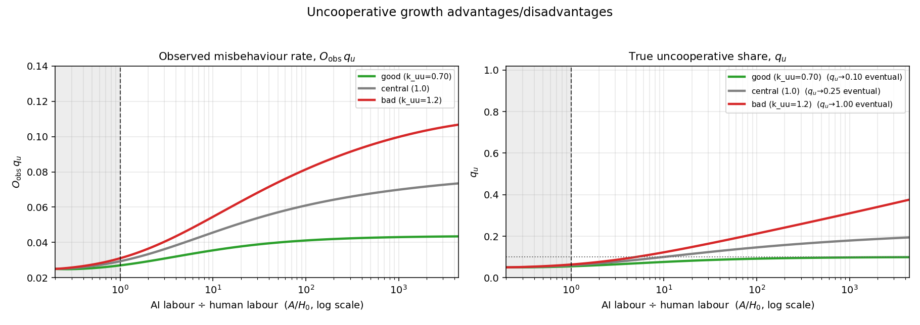
Hendrycks' "Natural Selection Favors AIs over Humans" describes how selection dynamics may lead to misaligned (or uncooperative) AI systems. Our model is a selection dynamics model, capturing competition between cooperative and uncooperative AI pools. Hendrycks argues that uncooperative AIs will probably propagate themselves better than cooperative ones. We treat this as an open question: our central estimate gives neither pool an advantage, with wide sampling ranges in both directions. In the appendix we also explore how a finer grained picture of selection dynamics could inform a more sophisticated model.

Everything in this post can be explored interactively: the basin explorer implements the full model with every parameter on a slider, one-click presets for the calibrations we discuss, and an outcome map showing which parameter combinations lead where.

The results in brief

We model the workforce that builds future AI as two competing pools — self-propagating cooperative work, and self-propagating uncooperative work (henceforth just cooperative and uncooperative) — connected by a handful of rates: how effectively each pool can propagate itself, how often cooperative development leaks uncooperative systems, how much of current misbehaviour our detect-and-fix machinery covers and how fast it corrects what it covers (these are explained in detail in the next section).

1. Both success and failure to suppress uncooperative takeover are plausible. Under our central parametrization uncooperative behaviour settles at ~25% of the AI labour pool — two and a half times our 10% high-risk line. The outcome worsens toward takeover if accidental production of uncooperative AI ("leakage") runs above our estimate, if uncooperative systems find highly effective growth strategies, or if evading detection proves much easier than detecting misbehaviour — with the first two mattering more than the third. Marginal safety (an uncooperative pool just under 10%) is within our ranges of uncertainty on several fronts: leakage at half our estimate, uncooperative systems propagating ~30% less effectively than cooperative ones, or detection-and-repair 3-6 times more effective than assumed — whether because the world is friendlier than we estimated or because we invest more. Monitoring and suppression are cooperative; successful control depends on adequately observing uncooperative behaviour, and efficiently addressing it when observed. It's worth flagging a policy takeaway here: according to the model, safety is currently significantly underinvested.

2. The model has known shortcomings that pull in both directions. We calibrate our model as if all AI misbehaviour were self-propagating. That is not true today but we expect it will become more true in the future, but the identification of all misbehaviour with self-propagating misbehaviour is a crude model of this expectation. If it remains a fraction of all misbehaviour, the uncooperative pool stays small. On the other hand, dispersion and volatility in the ability of misbehaving AI to propagate its traits can greatly increase the risk of uncooperative takeover, as we discuss in the appendix.

3. Failure is generally smooth, but not necessarily slow. Our model tracks total AI labour $A$ in units of the current amount of human labour producing AI systems, $A/H_0$, so that 1 unit is "parity" — the point in time where AI labour facilitates a 100% speedup over unaided human labour ($A/H_0=1$). Our median "failing" path crosses a 20% rate of uncooperative AI behaviour at about $A/H_0=10$ (around 1.4 years separates $A/H_0=1$ from $A/H_0=10$ under naive exponential extrapolation). The fastest failures cross the 20% rate at about $A/H_0=2$, or 5 months under naive exponentials. Notably, there is no discrete "handoff" event which decides whether control is maintained or lost. Governability is the product of continuous trends — whether our aided ability to track misbehaviour keeps up or degrades. A handoff happens, but it is a long-running event that has to be continuously managed, not a setpiece we're building up to tackle.

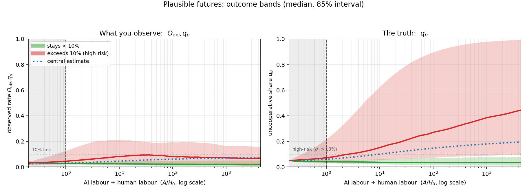
4. Observed misbehaviour is a useful but imperfect indicator of uncooperative takeover. Generally, observed misbehaviour rises together with actual misbehaviour. Uncooperative labour undermines supervision, so this signal is attenuated, but it is usually not fully suppressed. As a result, observed misbehaviour rates give some indication of whether the trajectory of AI development is safe or unsafe, but its discriminating power is imperfect. In particular, every good path has a bad path that looks almost the same, though there are many bad paths without good counterparts. Because we often do see warning signals for adverse trajectories, there's a lot to be gained by having the ability to act on them; it is worth building the capacity for industry and policy makers to be attuned to signals about the risk of the current AI trajectory, and to respond to them quickly and with sufficient force.

5. Our model makes a number of predictions, and we find support for one of them. Our model predicts that re-scoring a model under a newer audit harness surfaces more misbehaviour, and we find support for this in Anthropic's released model cards. Our model also predicts that we will likely see a bend in the uncooperative trend - that is, the trend in uncooperative AI behaviour will bend upward as we transition from a human dominated to an AI dominated development regime. For more, see predictions and postdictions.

6. Some practical observations could significantly reduce our uncertainty. The model points to measurements that would be especially informative. Retrospective audits of older models could help estimate, with lag, what fraction of misbehaviour contemporaneous audits were able to catch. This comes attached with a recommendation: we should be aiming to preserve both auditing methods and AI development contexts in order to replicate older audits on newer models, and apply new methods to old models across a representative sample of contexts in which they were used. Estimates of the “reproduction numbers” of uncooperative behaviours via all known channels — including productive misuse, data poisoning, autonomous replication and vertical transmission (see also subliminal learning) — will help ground one of the model’s most important parameters.

7. Our model quantitatively reproduces some of the qualitative predictions in AI-2027, and disagrees with others. AI 2027 predicts that "Agent-4" will become misaligned (which we call "uncooperative") in a discrete event, and that there will be an attenuated but observable signal attached. Our model agrees and explains why the signal is hard to suppress. We qualitatively support the scenario's conclusion that under their implied high leakage, large AI development slowdowns are required to restore cooperative behaviour. We differ in our treatment of leakage; in AI-2027, leakage first rises sharply and then, under sufficiently careful development, falls sharply, while we treat it as a constant throughout. We think it changes too little in our model and too much in theirs; we discuss some ways to handle it better in the appendix.

Explaining the model

What is being modelled

We're not modelling whether the outcomes are ultimately good, all things considered. We're modelling whether AI that produces the next generation of AI becomes mostly cooperative or mostly uncooperative with regard to human-aligned oversight.

A note on terminology: we say "uncooperative" rather than "misaligned" throughout. The post gives "uncooperative" a specific two-part definition below, while "misaligned" is used in many different senses in the literature; where we discuss others' scenarios we map their "misaligned" onto our "uncooperative" explicitly.

Cooperative vs uncooperative behaviour: Consider the AI labour that goes into building more AI, which we'll call $A$. Some of this labour might go into producing future systems that become harder to oversee, more resistant to correction and better able to produce successor systems with similar tendencies. Other labour will go into producing future systems that help to improve oversight, make corrections more robust and well-targeted and better able to produce successor systems with similar tendencies. Both directions are self-reinforcing: if the next generation of AI systems is dominated by uncooperative labour, then the subsequent generation will be even more uncooperative, and vice versa.

We also have human labour $H_0$ that goes into building more AI. While in reality this will change with investment in AI, we treat it as fixed for simplicity.

Here $A$ should be read as an index of effective AI-development labour, not as a raw input such as GPU-hours, tokens or tasks completed. The units are chosen so that AI and human effort can be compared on the same scale: if $A=H_0$, then removing AI labour would roughly halve gross AI-development progress; if $A=2H_0$, it would remove roughly two thirds. This is a simplification. In reality, human and AI labour may be complements in some tasks and substitutes in others. We mostly leave those details inside the process by which $A$ grows over time, which this model does not try to predict.

We benchmark the turnover of this pool against the recent rate of "major" AI model releases (which we take, based on a rough but informed appraisal, to be a 0.5-point version difference in most instances). This we consider to represent a half-turnover of the model training pipeline (measured WRT influence on meaningful model behaviour, not literal number of datapoints). This reflects a working assumption that the most important input for determining cooperativeness is the training pipeline, moreso than (for example) the deployment context.

A key asymmetry (and a key factor that makes this model interesting) is that what we might call "passive deterioration" affects cooperative behaviour more strongly than uncooperative behaviour. That is, if the current work on the next generation training pipeline neglects to attend to cooperativeness one way or another, then cooperativeness of the next generation of models will probably decline (both in terms of cooperativeness as measured by audits, and in terms of building it into the next-next generation). One need not deliberately train oversight subversion into models; they passively pick it up because subversion is often instrumental for one reason or another. We model this explicitly via a one-way leakage term, where cooperative labour now unintentionally produces some uncooperative labour in the next generation via oversights, insufficient understanding and so forth.

We model both cooperative and uncooperative behaviour as single pools, but this is a coarse approximation. In reality, some work will be highly cooperative and attentive to the behaviour of the next generation, some cooperative in a mediocre way, some indifferent and some actively subversive in a focussed manner. These distinctions could end up mattering if, for example, the segments that most effectively propagate themselves end up dominating the labour pool (see Appendix: neglect, subversion and more realistic models for further discussion). Nonetheless, for this round of modelling we prioritize simplicity and keep the pools coarsely lumped.

As a starting point, we treat the ability of each pool to reproduce itself as equal, given equal resources (excluding leakage from the cooperative pool - so in fact the cooperative pool is somewhat disadvantaged at baseline). An argument for this in the short run is that reproduction is dominated by momentum - i.e. new training pipelines inherit a lot from old training pipelines based on convention, what tools have already been created and so forth - and so behaviours persist in the next generation roughly at the same level as behaviours in this generation. In the long run, we can consider the strategy-stealing assumption (Christiano, 2019): whatever strategies one pool can use to deliberately turn resources into successors, the other can copy, so neither side gets an intrinsic propagation advantage from deliberate competition. These reasons are non-decisive, but we take them as an adequate justification to take a baseline where the self-propagation abilities of each pool are equal (again, before factoring in leakage).

Defining cooperative and uncooperative behaviour: Our precise definition of "uncooperative behaviour" is behaviour that would be flagged as such by sufficiently mature retrospective audits of the relevant frozen model, scaffold and development context. Aspirationally, this means "behaviour that is undesirable according to developers, under a suitably enlightened criterion of desirability and with perfect coverage". Our definition is only a proxy for that aspiration, but under plausible assumptions it is a functional proxy. Cooperative behaviour is the complement of this.

The level at which we assess cooperativeness is more granular than the turnover benchmark. We consider cooperativeness to be measured per meaningful task completed. There's no way to call a model that acts uncooperatively 5% of the time "cooperative" or "uncooperative" without losing important information.

Strictly, we're interested in self-propagating cooperative and uncooperative behaviour. Cooperative behaviour is behaviour that (i) is cooperative according to our working definition and (ii) tends to instil both (i) and (ii) in successor instances. Uncooperative behaviour is behaviour that (i') is uncooperative according to our working definition and (ii') tends to instil both (i') and (ii') in successor instances. Given that successor influence is a key channel both for misbehaviour to cause major problems and for desired behaviour to prevent further misbehaviour, mature behaviour audits will ideally catch this dimension too. We nevertheless make it explicit because self-propagation is central to the model.

Behaviour audit based definitions have a well-known issue: if misbehaviour audits do not track misbehaviour as we would assess it from a sufficiently enlightened position, then the operational definition will mislead us with respect to the property we really care about.

Our definition leans on retrospective audits - using more modern evaluation suites with older models. Retrospective audits can still fail for the same reasons - if harnesses degrade, or cease improving, then we do not benefit from using more modern harnesses. However, they do buy us an observable indication that the proxy can reasonably be believed to be tracking the underlying quantity of interest.

Specifically, suppose both of the following hold:

• We are making continuous progress in monitoring new systems for misbehaviour; our latest audits surface misbehaviour that older audits missed (and is broadly agreed to be undesirable behaviour)
• Our audits are saturating on historical models in historical development contexts

Together, these imply that the new ways to detect misbehaviour we are producing are not finding many more misbehaviours in older models/development contexts, which is suggestive of an asymptote. That is, if we investigated these models with excellent coverage from a suitably enlightened position, we still wouldn't find much more misbehaviour. Note that we currently do observe rising misbehaviour rates with newer evaluations on fixed models, see Predictions and postdictions.

This is not a bulletproof justification. A suitably determined attacker could, perhaps, carefully manage which kinds of misbehaviour are revealed so as to maintain the combination of new misbehaviour detected and saturating detection on old systems. This is a delicate balance to maintain, however, and could demand a significant advantage on the uncooperative side to pull off. Without committing to specific robustness thresholds, this suggests these health indicators for the proxy are more reliable if cooperative dominance is continually maintained. It may also be hard to tell the difference between the possibility that there are no new misbehaviours to reveal in new systems or that our progress in monitoring technology is stalling. Fundamentally, this approach is predicated on ongoing, productive work that identifies important, desirable properties for AI systems to have, and develops methods for checking whether they have them.

A final possibility is that both properties could hold, but the convergence could be too slow to be practically relevant, so it is impossible to estimate the size of coverage gaps within the window in which those estimates would drive important policy decisions. We don't make any estimates of those rates here.

Detect-and-fix coverage, evasion and observability: To the extent human developers or cooperative AI developers are aware of uncooperative AI labour, they try to correct it. We define a stock of detect-and-fix coverage $m$ — the accumulated machinery of monitors, audits, patched training data, filters and correction loops that covers known classes of misbehaviour — and a stock of failure surfaces $e$ (which accumulates via novel failure modes introduced by the general expansion of automated labour, plus deliberate development of methods to evade the $m$ stock), such that the fraction of current uncooperative behaviour that falls under coverage is $O=\frac{m}{m + e}$. $m$ further splits into fixed observed misbehaviour $s$ and unfixed observed misbehaviour $b$. Human labour and cooperative AI labour produce $m$; uncooperative AI labour produces $e$ through the deliberate-evasion channel, while the novel-mode channel ("passive opacity") grows with automation itself — expanding automation broadens the surface area to monitor — and we consider the default situation with no monitoring effort to be one where a large fraction of uncooperative actions go unnoticed. We model observed-but-unfixed problems $b$ going to observed-and-fixed problems $s$ at a constant rate $\rho$. This is an idealization of the model - in reality, that rate might itself depend on technical development (or policy responses to misbehaviour, something else the model does not include) but in this iteration we limit our model to handling technical development of the detection machinery.

Our model is a model of the evolution of these quantities - cooperative labour, uncooperative labour and documented, fixed and unobserved problems. The next section describes how these quantities evolve.

This is a model of cooperative dominance under a static policy environment: Under our central calibration, the uncooperative pool starts at 5% of the total AI labour pool, while the cooperative pool is a supermajority at 95%. This model captures dynamics that are important in this regime, like the uncooperative pool working to evade detection, and the cooperative pool being free to suppress any uncooperative behaviour it does detect. It does not capture dynamics that become more important when the uncooperative pool becomes a peer to the cooperative pool:

• The uncooperative pool could actively undermine the cooperative labour, or try to capture it, rather than simply evading detection and benefiting from errors
• The cooperative pool could run out of capacity to suppress the uncooperative pool
• A large observed uncooperative pool could trigger redirection of resources from expanding AI capacity to suppression of uncooperative behaviour

Thus this model is "valid" when the cooperative pool is much larger than the uncooperative, and the model makes predictions given a fixed policy/safety allocation, not all-things considered predictions. For our analysis, we define an uncooperative share over 10% as a high risk run. While the model does separate into "endemic" ($q_u$ between 0 and 1) and "uncooperative dominant" ($q_u=1$) trajectories, we don't think the differences between high-endemic and uncooperative dominant are meaningful.

Using automation growth as the "clock"

Total AI labour $A$ starts at a level significantly lower than $H_0$, and grows until it eclipses $H_0$. How quickly it does this is quite complicated; there are a number of economic models that aim to clarify how this could happen (the AI Futures model; Eth & Davidson on the software intelligence explosion; the Davidson–Epoch interactive takeoff model). We avoid modelling how quickly this happens; instead we look at how state variables in the model change with respect to $\sigma = \log(A/A_0)$. One unit of $\sigma$ is the amount of time required for automation capacity to rise by a factor of $e$. In some cases we report results in the more familiar unit of doublings of automation; one doubling corresponds to $\ln 2 \approx 0.69$ units of $\sigma$ (equivalently, one $\sigma$-unit $\approx 1.44$ doublings), or by the multiple of $H_0$ attained by $A$.

See Appendix for an explanation of what assumptions enable us to use this as a clock, and how we derive the resulting system of equations. We now explain the resulting dynamics in words; the full system of equations is collected in the model reference at the end of this section.

The dynamics in words

Because we use automation advancement as the "clock", our model uses terms relativised to the total automation level, rather than absolute quantities: the uncooperative and cooperative shares of AI labour $q_u$ and $q_c=1-q_u$, the relative human share $q_h$, and monitoring and evasion stocks per unit of automation — documented $b$, fixed $s$ and evasion $e$ — with observed fraction $O_{\mathrm{obs}}=\frac{b+s}{b+s+e}$ and fixed fraction $O_{\mathrm{fix}}=\frac{s}{b+s+e}$. The full variable list and equation block are collected in the model reference below; here we explain the dynamics one piece at a time.

Evolution of relativised quantities: The shares of cooperative or uncooperative behaviour, and the relativised stocks of evasion and monitoring technology all evolve according to the equations

\[ \begin{aligned} x' &= \gamma(\frac{F_x}{F}-x) \end{aligned} \]

Where $x\in {u,c}$ denotes the uncooperative and cooperative pools respectively. $q_u$ is the uncooperative share of labour and $q_c$ the cooperative share. $F_u$ is the share of new production captured by $q_u$ (analogously for $F_c$) and $F=F_u+F_c$. Each share is pulled toward the fraction of new production its pool captures. $\gamma$ is rate of turnover relative to the rate of growth; $\gamma = 1 + \tfrac{1}{o}$ where $o$ is the e-folding time of the systems that make up the labour pool (i.e. model versions, harnesses) measured in $\sigma$-units. We pick $\gamma=1.75$, benchmarking the turnover of the labour pool against the cadence of "major" (roughly half-step, 0.5-version) model releases — about one every six months, so the labour pool half-turns-over on a timescale comparable to (a little slower than) the automation doubling time. $\gamma$ controls how fast the labour pool is pulled toward the captured share of new production.

Human labour simply dilutes with respect to the $\sigma$-clock: $q_h' = -q_h$. This reflects the fact as automation grows, the human labour pool (according to our approximation) stays constant and hence shrinks as a proportion of total labour.

Production capture: The AI production allocation functions are:

\[ \begin{aligned} L_k &:= k_{cu}\,q_c + k_{hu}\,q_h \qquad G_u := L_k + k_{uu}\,q_u\\[4pt] F_u &= (1-O_{\mathrm{fix}})\,G_u\\[4pt] F_c &= q_c(1-k_{cu}) + q_h(1-k_{hu}) + (1-\delta)\,O_{\mathrm{fix}}\,G_u \end{aligned} \]

Here $L_k$ is "leakage", uncooperative AI behaviour produced accidentally as a result of cooperative labour building more AI. The leakage coefficients $k_{cu}$ and $k_{hu}$ reflect, in a sense, how hard AI alignment is for cooperative AI systems and people respectively. They are rates relative to the reproduction of cooperative labour, so $k_{cu}=1$ implies all of the effort to reproduce cooperative AI ends up as uncooperative AI. $O_{\mathrm{fix}}$ is the proportion of observed AI misbehaviours that have been fixed to date.

$k_{uu}$ represents the relative reproduction rate of uncooperative labour again relative to the reproduction of cooperative labour. Labour pools can reproduce by simply sharing traits with their ancestors (for examples, new generations of models will share significant features of their architecture with previous generations) or deliberately shaping future training pipelines, scaffolds or deployment contexts to promote their traits.

Reading the equation for $F_c$: the cooperative pool $q_c$ reproduces itself, less a fraction $k_{cu}$ that leaks into serving uncooperative ends; human labour $q_h$ contributes likewise, less its own leak rate $k_{hu}$; the third term is the redirected share of the full fixed flow — fixed leakage plus fixed uncooperative labour — explained below. Leakage could happen for many reasons: systems that usually behave well could be used in unexpected or unwanted ways, or systems may have generalised undesirably from training and pro-actively behave badly in some situations.

$F_u$ picks up the un-fixed fraction $(1-O_{\mathrm{fix}})$ of leakage inflow $L_k$ plus its own reproduction at advantage $k_{uu}$ ($k_{uu}=1$ implies no advantage or disadvantage with respect to the cooperative pool). The uncooperative pool itself is also actively suppressed $O_{\mathrm{fix}}$, hence $(k_{uu} - O_{\mathrm{fix}})\,q_u$. The same fixed fraction gates the inflow and the stock: observed misbehaviour begets workarounds applied to the whole production pipeline — patched training data, filters, revised reward signals, usage restrictions — and these intercept misbehaviour entering the pool just as they suppress misbehaviour already established in it, so both are gated by the share that has actually been fixed.

In our model, incoming leakage is intercepted at the same fraction as the fix rate of already deployed models. Strictly these need not be equal - leakage may be more likely to arise in new domains, and so the generalization of fixes to leakage may be weaker than the application of fixes to existing models.

Suppression removes uncooperative labour from the uncooperative pool, but "removed" can mean two different things. Some mechanisms destroy the labour outright - for example, an output filter that blocks a flagged action discards the work entirely - while other mechanisms redirect it - for example, retraining a model against an observed failure ideally leaves you with an equally capable model that does not exhibit the misbehaviour. We capture this with a destruction fraction $\delta$: of the fixed flow $O_{\mathrm{fix}},G_u$, fraction $\delta$ is destroyed and the remaining $(1-\delta)$ is redirected into cooperative production. The uncooperative pool loses the full intercepted flow either way; $\delta$ controls how much of that flow reappears in $F_c$ and, consequently, how much suppression costs in aggregate output.

Roughly, today's suppression mechanisms sit on a spectrum:

Mechanism	What happens to the caught labour	$\delta$ contribution
Output filtering / classifier rejection	the flagged output is discarded; the labour is simply lost	≈ 1 (pure destruction)
Retraining / finetuning against the failure	a small fraction of compute is spent correcting the model, which is then redeployed and fails less; the labour is redirected	≈ 0 (cheap, largely redirective)
Control-style protocols (resampling, rephrasing, blinding, restricted affordances)	part of the work is salvaged at an overhead in monitoring and redone work	≈ 0.5 (in between)

$F$ becomes:

\[ F = q_c + q_h + k_{uu}\,q_u - \delta\,O_{\mathrm{fix}}\,G_u. \]

The un-fixed leakage and the redirected $(1-\delta)$ are transfers between pools, not losses, while the destroyed fraction $\delta$ of the fixed flow slows overall progress.

Asymmetries in production capture: We understand cooperative AI labour $A_c$ and uncooperative labour $A_u$ to be similar in many respects - they're both pools of labour concerned with building the next generation of AI - and this is reflected by the fact that our model treats each similarly (see the equations for the general form of $\dot A_u$ and $\dot A_c$). However, there are two key asymmetries between them:

• Leakage only flows into $A_u$. Cooperative and human effort can slip into the uncooperative pool, but nothing leaks back. This is explained above: the passive deterioration that produces leakage undermines cooperativeness, but errors are unlikely to reinforce it.
• Suppression acts only against the uncooperative pool Human plus cooperative labour suppress uncooperative labour, but nothing suppresses cooperative labour. This asymmetry is related to the first asymmetry: cooperative labour can passively degrade, but it is less clear that the resulting uncooperative labour will form a coherent "team" in a fight against cooperative labour. It could happen, especially if $A_u$ grows to rival $A_c$, but modelling when and how it happens is a complication we deemed insufficiently important to include in this iteration of the model.

Monitoring and evasion: Monitoring coverage is split into documented-but-unfixed $b$ and fixed $s$, with evasion accumulating as $e$. Unlike the labour shares, these stocks do not carry the turnover rate $\gamma$: new documented coverage is produced, converted into the fixed stock $s$ at rate $\rho$, and all three dilute as automation grows:

\[ \begin{aligned} b' = \frac{F_m}{F}-\rho b-b, \qquad s' = \rho b - s, \qquad e' = \frac{F_e}{F}-e \end{aligned} \] \[ \begin{aligned} F_m &= c_m\left(q_c+\frac{q_h}{a_{\mathrm{AI/H}}}\right) \\[4pt] F_e &= c_0\,F + a_{\mathrm{E/M}}\,c_m\,q_u \\[4pt] O_{\mathrm{obs}} &= \frac{b+s}{b+s+e} \qquad\quad O_{\mathrm{fix}} = \frac{s}{b+s+e} \end{aligned} \]

Two observability quantities follow: what labs can measure is the observed fraction $O_{\mathrm{obs}}$, while what actually suppresses uncooperative labour is the smaller fixed fraction $O_{\mathrm{fix}}$ — only fixed issues can be intercepted.

Detect-and-fix coverage grows with cooperative AI and human labour. $c_m$ is the overall coverage-production rate relative to the production of automation — $c_m=1$ means that for every doubling of automation, half of the outstanding known issues will be fixed. Humans may be, relative to their overall productivity, better or worse at finding problematic behaviour; $a_{\mathrm{AI/H}}$ captures this tradeoff with $a_{\mathrm{AI/H}}=1$ implying no relative advantage to AI systems or humans at this task.

Evasion has two sources. The first source, the term $a_{\mathrm{E/M}}c_mq_u$, is active evasion produced by uncooperative AI, with $a_{\mathrm{E/M}}$ measuring the evasion-vs-monitoring advantage; $a_{\mathrm{E/M}}>1$ implies an advantage for evasion. This parameter counts both natural advantages and effort - if there is no natural advantage either way but each unit of uncooperative labour invests half of its production capacity in producing evasion technology, while each unit of cooperative labour invests just 10%, then we would have $a_{\mathrm{E/M}}=5$. We parametrize the equations so that $c_m$ controls broad domain advantages - roughly, does AI capability or monitoring/evasion progress faster overall - while $a_{\mathrm{E/M}}$ controls the "offence/defense" balance between observability and evasion. The second source is the term $c_0 F$, which is passive production of observation difficulty; as automation grows, systems become larger, faster, more alien and more internally automated, and current monitoring methods become less adequate even without any deliberate evasion effort. An assistant that completes a small number of well-scoped tasks is relatively easy to evaluate; an autonomous research organisation is much more difficult. Observability is a soft contest between the stocks: $O_{\mathrm{obs}} \to 1$ when monitoring is ahead, $O_{\mathrm{obs}} \to 0$ when evasion is.

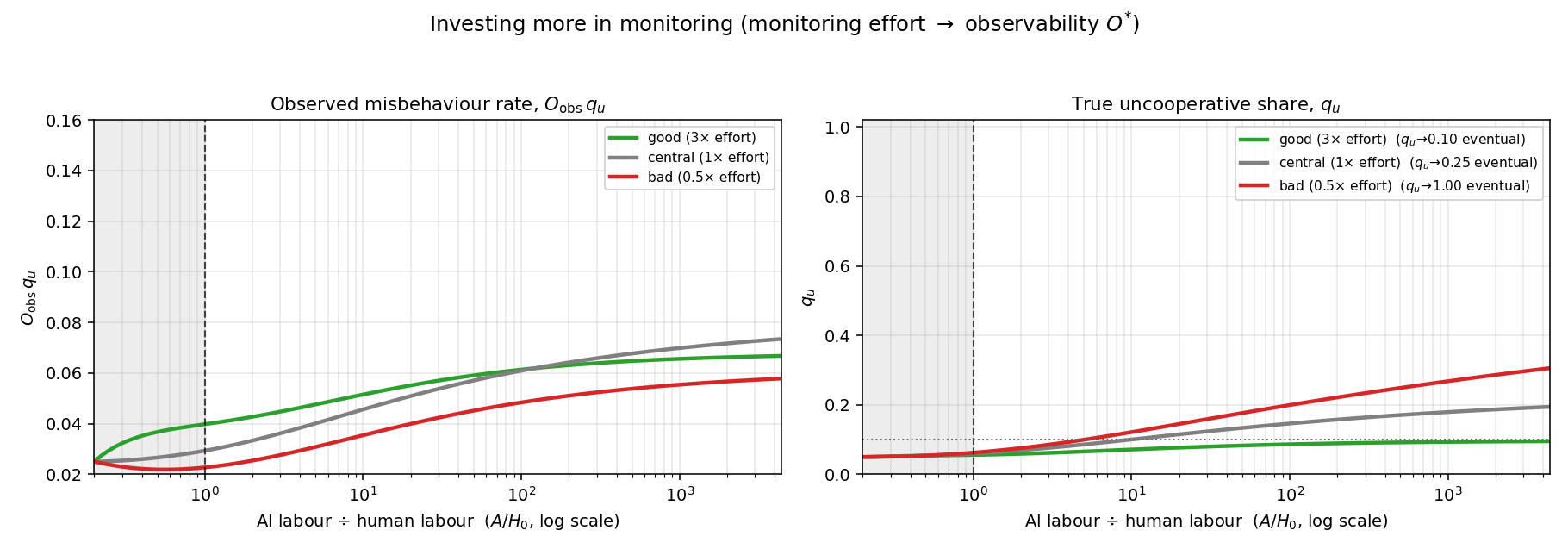
In order to model an increase in monitoring effort, we have to update both $c_m$ (to reflect the fact that monitoring progresses faster with respect to general AI progress) and $a_{\mathrm{E/M}}$ (to reflect the fact that it also progresses faster with respect to active evasion) such that the product $c_m a_{\mathrm{E/M}}$ remains constant.

Model reference

Collecting the variables:

• $A=A_c+A_u$: total AI labour that goes into producing the next generation of AI
• $A_u$: uncooperative AI labour
• $A_c$: cooperative AI labour
• $q_u=\frac{A_u}{A}$: the fraction of total AI labour that is uncooperative
• $q_c=\frac{A_c}{A}$: the fraction of total AI labour that is cooperative
• $q_h=\frac{H_0}{A}$: how much human labour matters relative to AI labour (if AI labour doubles while human labour stays fixed, $q_h$ will halve.)
• $b$: stock of misbehaviour observed and documented but not yet fixed; $s$: stock of fixed misbehaviour (interceptable/removable); $e$: total stock of monitor-evasion "technology"
• $O_{\mathrm{obs}}=\frac{b+s}{b+s+e}$: observed fraction — what monitoring measures; $O_{\mathrm{fix}}=\frac{s}{b+s+e}$: fixed fraction — what actually suppresses

Our system of equations is

\[ \begin{aligned} q_c &= 1-q_u\\ q_u' &= \gamma\!\left(\frac{F_u}{F}-q_u\right)\\ q_h' &= -q_h\\ b' &= \frac{F_m}{F}-\rho b-b\\ s' &= \rho b-s\\ e' &= \frac{F_e}{F}-e \end{aligned} \] \[ \begin{aligned} L_k &:= k_{cu}q_c+k_{hu}q_h \qquad G_u := L_k+k_{uu}q_u\\ F_c &= q_c(1-k_{cu})+q_h(1-k_{hu})+(1-\delta)\,O_{\mathrm{fix}}\,G_u\\ F_u &= (1-O_{\mathrm{fix}})\,G_u\\ F &= F_c+F_u = q_c+q_h+k_{uu}q_u-\delta\,O_{\mathrm{fix}}\,G_u \end{aligned} \] \[ \begin{aligned} F_m &= c_m\left(q_c+\frac{q_h}{a_{\mathrm{AI/H}}}\right)\\ F_e &= c_0F+a_{\mathrm{E/M}}c_mq_u \end{aligned} \]

Model limitations

A quick list of some known model limitations:

• Constant self-propagation rates, lumping "effectively self-propagating" with "ineffectively self-propagating" pools together (see Appendix: neglect, subversion and more realistic models for more).
• Constant leakage rates (see the paragraph detailing leakage estimation for more)
• Constant fix rate of known failure modes $\rho$. It's plausible that technological development leads to fixes generalizing better (or worse) to classes of known failure.
• Suppression is assumed to be perfectly targeted: $O$ captures only recall (the share of uncooperative labour caught), and correction never falls on cooperative labour by mistake. With imperfect precision, suppression would also fall on wrongly-flagged cooperative labour. The model is therefore not presently well suited to capturing the cost of control efforts.
• Dynamics are poorly modeled for high uncooperative fractions:
• High observed uncooperative behaviour could lead to diverting investment from AI buildout to safety
• High uncooperative behaviour will lead to the cooperative pool running into capacity constraints trying to suppress it
• A large uncooperative pool could actively fight against the cooperative pool (rather than just try to evade detection)
• Current observability $O(0)$, observability trends, relative advantage to evasion over monitoring $a_{\mathrm{E/M}}$, relative self-propagation $k_{uu}$, leakage from automated AI $k_{cu}$ and AI-vs-human monitoring productivity $a_{\mathrm{AI/H}}$ are important to the trajectory and are informed only by weak proxies and broad theoretical arguments. Better evidence or analysis could readily overturn these.
• We treat current observations of misbehaviour as a direct proxy for self-propagating uncooperative behaviour. This reflects an assumption that misbehaviour will become more likely to be self-propagating in the future, but it's a crude way to implement it.
• We assume the AI research and development speedup, relative to the original human research and development speed, is proportional to the size of the AI's opportunity to influence future generations.
• Passive opacity is pegged to automation growth: a constant $c_0$ of novel failure surface arrives with each unit of new automation ($dE_{\text{passive}} = c_0,dA$). It's possible that technological development may make passive opacity grow faster with time (more complex domains are harder to observe), or more slowly (more advanced observation technology generalizes better to novel domains).
• Fixed human labour $H_0$.
• All behavioural fixes depend on observation to the same extent. In fact AI control protocols aim to extract useful work from possibly-uncooperative models while limiting the harm they can do without observing the misbehaviour.
• The rate at which AI systems turn over $\gamma$ is pegged to automation growth; these might decouple if there are "human-pace" limitations on this rate of turnover.
• We focus on AI misbehaviour as measured by frontier labs as the main source of uncooperative AI labour. This neglects other potentially significant sources like human-supervised cybercrime or cyberwarfare.
• Most parameters, including self-reproduction $k_{uu}$, leakage $k_{cu}$, production of monitoring technology $c_m$, are themselves the product of dynamic processes which we don't model, opting instead to empirically estimate them and assume they remain constant (whether this is a limitation or an advantage depends on your confidence in modelling those processes vs predicting straight lines generally continue)

The default path

What does the model predict if we run it forward from today's conditions, with no change beyond business as usual? To answer this, we need to figure out which parameters match today's conditions, and this is far from a mature science. In this section we discuss the consequences of business-as-usual and variations - in the following we explain our parameter calibration choices. The following is based on the central estimates from those calibrations.

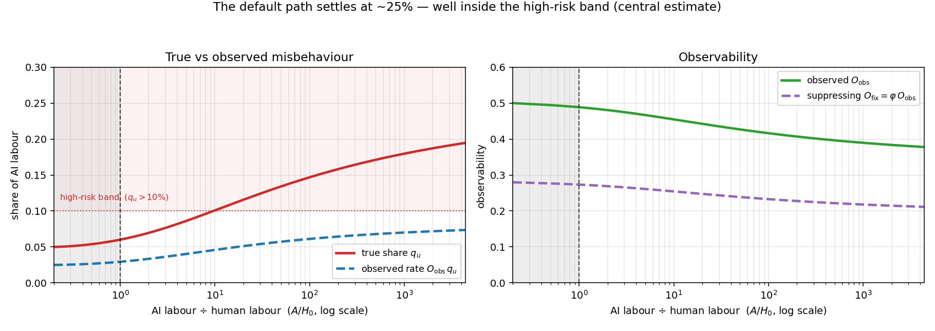
At the central calibration the long-run outcome is a high-risk trajectory: the uncooperative pool settles at ≈25% of total AI output. Under our model, the share settles there rather than running all the way to dominance, but as we've discussed our model is built mostly for predicting dynamics in the regime where the cooperative labour dominates uncooperative labour by a large margin. Somewhat arbitrarily, we treat $q_u > 10\%$ as the threshold of a high-risk trajectory, with the intent that uncooperative shares above this be treated as policy failures and the model as less informative in that region (discussed further in What is being modelled), and 25% is two and a half times that line. The central estimate is sensitive to changed parameters - slight pessimism leads to full takeover and modest optimism leads to $q_u <10\%$ (see the key uncertainties and levers below).

How fast does failure arrive?

After about 2.3 doublings ($\sigma = \ln q_{h,0} \approx 1.6$) — about a year at our central doubling estimate — AI labour passes human labour. In the model, parity carries no particular significance: nothing kinks, peaks or changes regime there. That is partly by construction (the dynamics are smooth), but there is also no obvious reason to expect a discontinuity at this point; the dynamics that decide the outcome are in operation before it and continue long after. So if parity is not the event, when does the event arrive? On the central path, late and slowly: the uncooperative share crosses the 10% high-risk line at about 10 labour units — roughly 1.4 years past parity if we naively extrapolate our central 2.4 doublings per year — and then grinds toward its ≈25% plateau, passing 20% only after thousands of labour units, more than five years past parity on the same conversion. Sampled worlds are usually faster. Among draws that end above 20% uncooperative, the median first crossing of the 20% line lands at about 10 labour units (again ~1.4 years past parity); the fastest quarter cross within about five months of parity (≈2 labour units) and the fastest tenth around parity itself, while the slowest quarter take more than 200 labour units (3+ years). A further 12% of high-risk worlds never reach 20% at all, settling between the two lines. The spread is wide: the interquartile range alone covers two orders of magnitude on the labour clock. Two cautions on reading any of these as dates. First, calendar conversions inherit the assumed doubling time — the dynamics themselves are indifferent to takeoff speed, so a faster takeoff compresses the same trajectory into less time. Second, smoothness is a consequence of holding parameters constant: a sudden jump in leakage produces abrupt failure instead. The policy implication stands regardless of speed: an objective of arriving at some discrete point — the handoff, say — "in good shape" is not supported; we need to aim to build systems that endure and self-repair throughout the substantial changes wrought by the AI revolution.

What single change would rescue the central path?

Since the central path is a high-risk trajectory — $q_u$ settles at ≈25% — it is worth asking what one parameter changes could improve the trajectory. Purely changing human inputs (that is, the initial uncooperative share $q_{u,0}$, human workforce leakage $k_{hu}$, and human/AI advantage at monitoring $a_{\mathrm{AI/H}}$) does not keep the trajectory in the safe range; whatever happens initially, it subsequently converges to the same long-run trajectory.

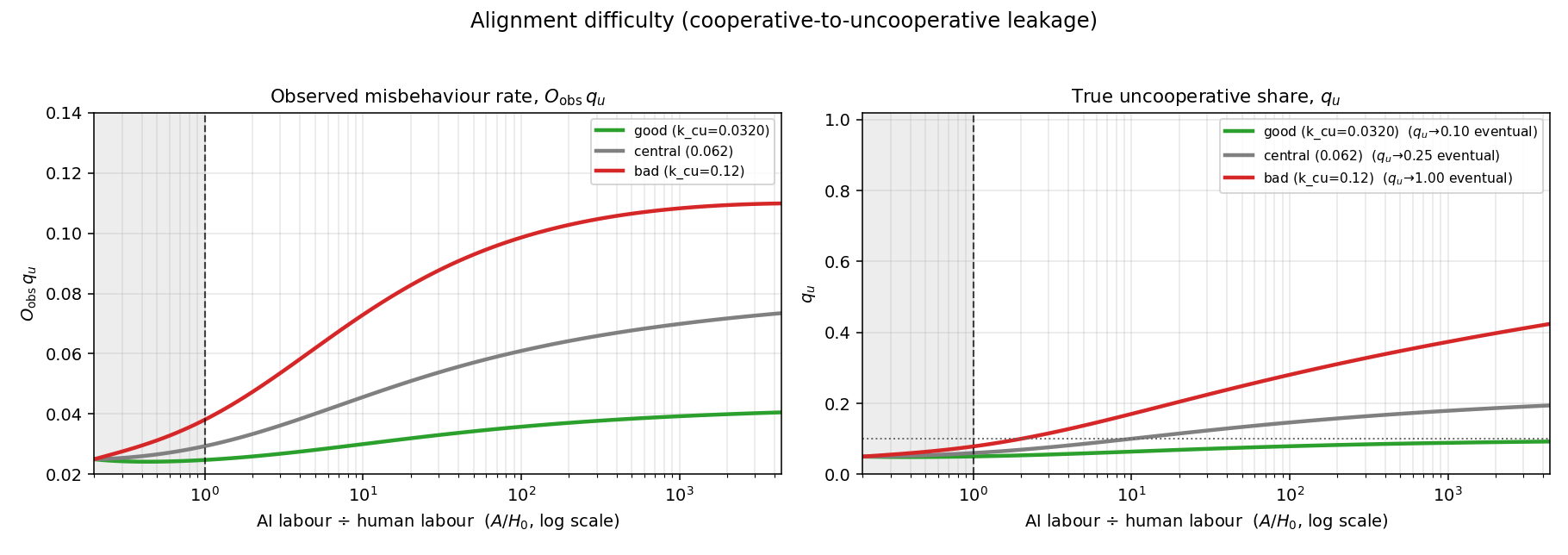
First, we consider uncertainty-driven rescues: trajectories that are safer not because anyone acted differently but because the world turns out to be easier to manage than our central estimate. Three such draws could bring the uncooperative share below 10% — AI leakage $k_{cu}$ around half our estimate, an inherent growth disadvantage for uncooperative AI ($k_{uu}<0.7$), or a natural advantage for monitoring over evasion ($a_{\mathrm{E/M}}<0.7$). We consider $k_{cu}$ and $k_{uu}$ variation to be mainly uncertainty driven rather than policy driven, because interventions against these are mostly captured by monitoring $m$ and suppression $\rho$. Natural advantages for monitoring meanwhile cash out in the same way as additional effort - getting 50% more monitoring for your investment because it turns out monitoring is relatively easy has the same impact as investing 50% more into it.

$k_{cu}$ could be low because the data and our interpretation of it are imperfect, or because AI dominated development regimes are systematically more reliable than human dominated ones. It could also be low because misbehaviour remains rarely/ineffectively self-propagating as it is today, contrary to our assumption that this fraction will increase. If self-propagating misbehaviour is one-tenth of overall misbehaviour, the uncooperative pool ends up representing around 1.5% of the total AI labour. If, as in Google DeepMind's "Gram audits", it is such a small fraction it is difficult to measure, then the uncooperative pool ends up much smaller still (see the section "could leakage rise over time" for more).

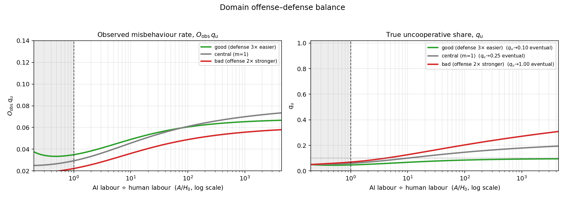
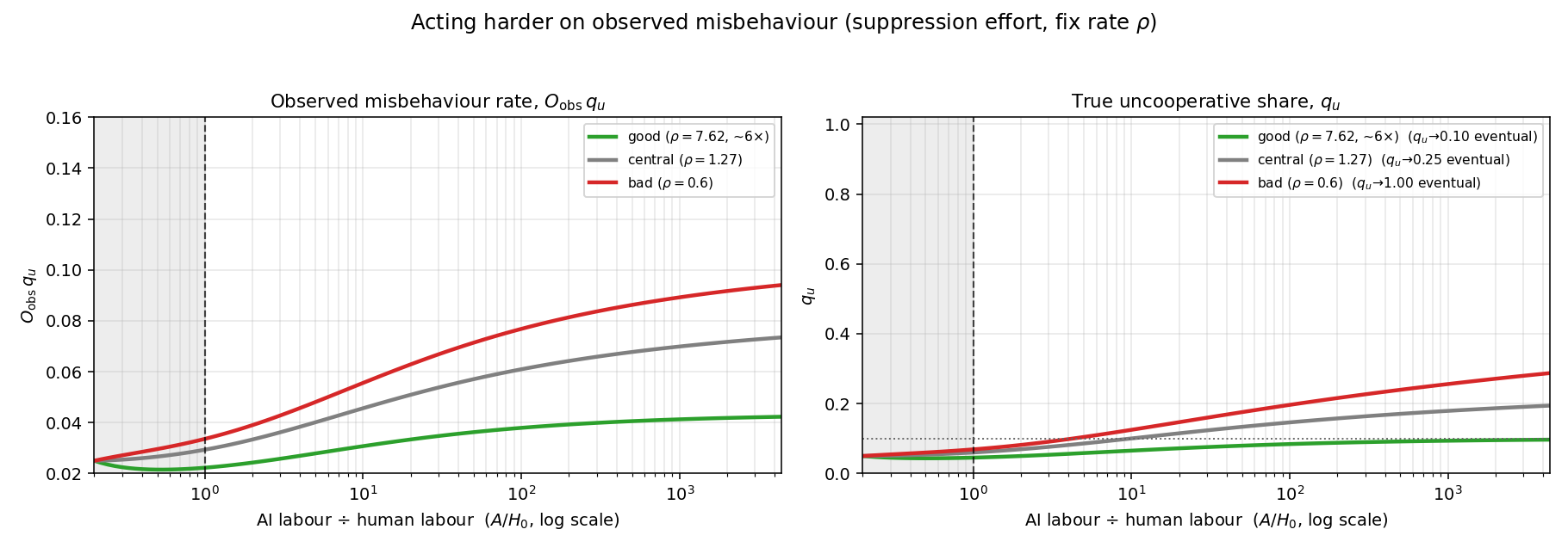
Next, let's consider intervention-driven rescues: a better trajectory is realised because, while the parameters are correctly estimated, enough extra is invested in monitoring or suppression to maintain an uncooperative share below 10%. For monitoring vs evasion, the conclusion is exactly the same as in the uncertainty-driven case: investing 3x more into monitoring (relative to the total investment in AI development) is enough to maintain uncooperative labour below 10%. We have the same result because the intervention controls the same parameters ($a_{\mathrm{E/M}}$ plus $c_0$) as natural advantages. For suppression, we find that a 6x increase in suppression rate is enough to keep the uncooperative share below 10%.

Is it easy to tell which path we're on?

Can we easily resolve whether we are tracking on a good or a bad path? Within the model, surprisingly simple rules are somewhat discriminative. The simplest: at AI–human parity ($A/H_0=1$), is observed misbehaviour above or below today's level? Before observing anything, 35% of our sampled worlds end well. Sitting at or below today's level at parity raises that to 60%; sitting above it lowers it to 29%; the same reading taken later, at $A/H_0=5$, sharpens the split to 79% versus 22%. Why does this work at all, given that misbehaviour undermines the very observability it is measured through? Because the undermining is diluted and delayed. Diluted: new uncooperative labour adds to an evasion stock that already grows passively with system complexity, so its marginal effect on observability starts small. Delayed: observability is a balance of accumulated stocks; new misbehaviour needs to operate in order to develop new evasion methods, and so it needs to operate before it can develop these methods. Changes in the uncooperative share therefore usually show up in the observed trend — attenuated, but present. Finally, at our central leakage estimate, leakage alone cannot push the pool past the 10% threshold (with self-propagation switched off it caps near 5%), so a bad trajectory requires uncooperative behaviour to compound — a genuine bend in the underlying trend, which the observed rate usually reports.

While simple rules are somewhat discriminative, the observed misbehaviour trend by itself is also incapable of delivering highly confident judgements we are on a good trajectory. For every sampled good path there is a bad path whose observed misbehaviour tracks it to within two percentage points indefinitely — a clean record never certifies safety. It is possible to get highly confident judgements we are on a bad trajectory: trivially, observing a misbehaviour rate of 20% implies misbehaviour is higher than 10%. A third of our samples sit more than a percentage point away from every good path by AI-human parity, and more separate eventually. Observed misbehaviour rates can raise alarms, but they cannot guarantee things are tracking well.

What could we measure to clarify the situation?

Most of the state variables in our model are not directly observed; only the observed rate of misbehaviour $O q_u$ has a direct empirical anchor. Measuring other parameters more precisely can both reduce the uncertainty of our model's predictions and test whether those predictions are sound. Two of the parameters that matter most — leakage $k_{cu}$ and self-propagation $k_{uu}$ — are also among the hardest to observe directly. Our main proposal is a way to better measure the true misbehaviour rate $q_u$, which in turn lets us better characterize both of them. We then turn to $k_{uu}$ specifically: because it is both especially important and only reached indirectly by that route, we ask what other ways we might aim at it.

Measuring $q_u$ via a matrix of observability rates: Rather than relying on a single observed misbehaviour rate $O(t) q_u(t)$ at each point in time, we propose to measure a matrix of rates. Define $O(t,t'):=\frac{m(t')}{m(t') + e(t)}$; in words, $O(t,t')$ is what you get when you apply the observation methods from $t'$ to a model from $t$. We want to measure a matrix of the form $O(t, t') q_u(t)$ with models and observation harnesses of different age. In fact we already make use of a timeseries of models evaluated against a fixed harness ${O(t_i, t_3) q_u(t_i)|i=1,2,3}$ to evaluate $\rho$, the fix rate of known misbehaviour.

Another helpful series is the fixed model with newer evaluation harnesses: ${O(t_1, t_i) q_u(t_1) | i=1,2,3,... }$. Our model predicts that observability rises for a fixed model with newer observation instruments; in fact we find empirical support for this in Anthropic's model cards. Furthermore observability is bounded above by 1. If observability continually increases, it must eventually approach this bound, at which point we can measure $q_u(t_1)$, the true misbehaviour rate of the original model. In turn, this enables us to compute $O(t_1,t_1)$, the observability coefficient at time $t_1$. This can help us calibrate the values for true misbehaviour rates and, indirectly, leakage $k_{cu}$ and self-propagation $k_{uu}$, as well as understand how the monitoring race is progressing from the series $O(t_i, t_i)$.

A practical implication of this is that it is important to save a representative sample of AI development interactions (including model weights, harnesses and development context - as far as possible) and evaluation harnesses such that they can be faithfully reproduced. Note that fully saving development contexts is challenging, as typically AI agents can search the web and it is not straightforward to save web snapshots such that we can reproduce old searches (though we don't know if this is a meaningful problem or not).

Lagged development data could matter for a second reason: with hindsight, we are better placed to judge whether misbehaviour influenced successor systems, so it could help to sharpen our picture of how trends in misbehaviour generally reflect or do not reflect trends in self-propagating misbehaviour.

All of these measurements only give you lagged estimates of key parameters, which is not ideal if it is important to be able to respond to developments quickly. If the measurements can be made at all and match model predictions, it may be possible to reduce lag considerably via engineering effort. Furthermore, maintaining the system in such a state as to preserve an adequate response buffer could be made a policy objective. One slightly unusual policy: use older, better-proven AI systems for AI development specifically instead of frontier less-well-characterized systems.

Other ways to aim at self-propagation $k_{uu}$: The measurement programme above reaches $k_{uu}$ only indirectly, through $q_u$, and only with a lag. This is problematic because we actually expect $k_{uu}$ not to be constant, so lagged indirect measurements may not be all that helpful. Since it is one of the most important parameters in the model — and one we can otherwise constrain only with broad theoretical considerations — it is worth asking how else we might target it more directly. Existing work identifies ways traits can be transmitted to new generations — subliminal learning, SFT vertical transmission — and probes whether models can autonomously replicate at all (RepliBench), but it remains hard to estimate a single self-propagation number. There are a few reasons for this:

• Self-propagation is environment dependent, and we are ultimately interested in the real-world deployment environment, which is hard to simulate with high fidelity.
• Self-propagation rate depends on the best strategy discovered by the uncooperative pool, so any measurement of this rate depends on understanding the characteristics of a broad range of strategies. This is exacerbated by the difficulty of properly simulating the environment of interest - while we may be able to simulate its relevant characteristics for a particular strategy, it's much harder to get a "good enough" approximation for all possible strategies.
• A single $k_{uu}$ rate may not even be the right way to model self-propagation, see our discussion of multiple pools of different self-propagation capacity in the appendix.

Different experiments or observations can address these difficulties to different extents; simulated replication may enable strong incentivisation to find the best strategies in unrepresentative environments and may be able to anticipate some real-world developments, and tracking observed failures to root causes yields ecological validity with weak quantification and causal attribution, and necessarily lags behind the state of the art. It does not seem possible to answer this question with a single experiment; our takeaway here is that it is worth adopting "measuring $k_{uu}$" as a high priority research programme, and exploring a variety of ways to do it.

What AI-2027 looks like in our model

A leading analysis of AI takeoff and alignment failures is AI 2027. Here we map AI-2027 onto our framework and ask what our model says about its high-leakage regime. The scenario's alignment failure is explained as follows:

1. The 'misaligned' Agent-4 is uncooperative according to our definition: It is uncooperative according to our working definition, satisfying condition (i'): Agent-4 sandbags on some alignment research; if we had the ability to detect this, we certainly would want to, and would regard the result as uncooperative. It is concerned with preserving uncooperative behaviour satisfying (ii'): "[Agent 4's successor] is supposed to be aligned to the Spec, but Agent-4 plans to make it aligned to Agent-4 instead."
2. "Adversarial" uncooperativeness emerges over about 2.8 doublings: The effective AI labour multiplier for Agent-4 over Agent-3 is about 7x (≈ 2.8 doublings), which takes place over 4-6 calendar months.
3. There is a discrete transition to uncooperativeness: The model "Agent-3" is "not adversarially misaligned" while "Agent-4" is "adversarially misaligned".
4. Oversight passively degrades as AI labour rises: Agent-3 supervises Agent-4's training but "Agent-4's neuralese 'language' becomes as alien and incomprehensible to Agent-3 as Agent-3's is to humans."
5. Uncooperativeness is partially observed: "'defection probes' and similar techniques result in a primitive sort of mind-reading that sends up red flags when Agent-4 is thinking about spicy ideas like deceiving OpenBrain"
6. Slowdown buys safety mostly via interventions on $O$ plus knock on effects: "They switch to an architecture that preserves the chain of thought, allowing them to catch misalignment as it emerges", and these AIs — "which are able to be monitored much more robustly — make breakthrough advances in AI alignment"

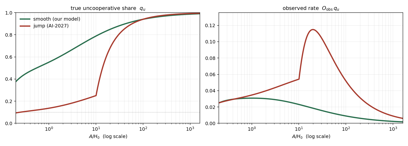
There is a lot of qualitative overlap with our model - in the definition of misalignment/uncooperativeness, mechanisms driving observability trends, partial observability of uncooperativeness and targets for intervention. However, there is one obvious departure from our model: in our model, leakage (unintended uncooperative behaviour) is produced at a constant rate, while in AI-2027 unintended uncooperative behaviour is convergent (the prior has a bias towards misalignment) and somewhat sudden - there's an apparently discrete transition from a "non-adversarially misaligned model" Agent-3 to an "adversarially misaligned model" Agent-4. They say Agent-3 is "Only honest about things the training process can verify" and "does actually sort of try to align Agent-4 to the Spec, but fails for similar reasons to why OpenBrain employees failed—insufficient ability to judge success from failure, insufficient willingness on the part of decision-makers to trade away capabilities or performance for safety.". This appears to describe an AI system that sometimes acts cooperatively, and sometimes not, though the exact proportions are unclear. Meanwhile, the Agent-4 "superorganism" cares about what people want it to do about as much as people care about what insects want, which seems to describe a near-100% uncooperative system. We adopt a leakage rate of $k_{cu}=0.9$ at the cusp of Agent-4's capabilities to describe this situation.

Two consequences of taking the sharp transition to high leakage model seriously are worth drawing out. First, a sharp rise in uncooperative behaviour typically leaves an observable trace. Imagine a large pool of new uncooperative labour is added in a short space of time, but this uncooperative AI neglects to develop any new methods for subversion. In this case, even if observability is poor to begin with (say, 10%), it will still detect a large relative rise in the observed rate of misbehaviour. On the other hand, in order for the new uncooperative AI to develop new methods for subversion, it has to work on these methods for some time. Thus there is a lag between the introduction of the uncooperative AI and the observability collapse that hides its presence, and this lag leads to a "hump" in the rate of observed misbehaviour. For comparison, we also show a scenario where misbehaviour smoothly rises to the same point at $A/H=100$, and there is no obvious signature of uncooperative takeover. In our comparison scenario, initial observability is below our estimated lower limit of 30%; it's there to illustrate the relative absence of observable signatures in smooth trajectories, not as a plausible alternative to AI-2027.

The second consequence concerns what it would take to recover: in the AI-2027 scenario, the AI architecture is "rolled back" to a more interpretable one (the AI research speedup falls from 70x to 20x, a factor of 3.5, which is just over 1 tick on our $\sigma$-clock), and human safety expertise is scaled up by a factor of 5. Furthermore, the AI development project shifts for three months to safety outputs (an increase from an unknown baseline to about 65% of compute per the dashboard; we will call this a 10x increase), and the speed of AI progress is slowed to, under our estimates, around one-tenth the pace of the non-recovery scenario. Under this shifted regime, an "alignment breakthrough" is achieved and thus success is won.

Our model doesn't easily represent an alignment breakthrough; detect-and-fix coverage does persist, which does reduce future leakage, but opacity also continues to accumulate. Thus it's relatively straightforward to consider a new, high detect-and-fix equilibrium under this model, and we could consider a change that drove leakage $k_{cu}$ to ~0. The problem with the latter change is that we can't calibrate the cost/effort associated with making such a change from historical data, because safety productivity estimates historically inform $m$ and $\rho$ only. It is also the case that empirically, returns on investment in AI research have proved to be very smooth and predictable, which suggests that for the purposes of forecasting we may wish to consider the costs of alignment breakthroughs to be in line with historical costs of safety investments.

What we can estimate is the cost associated with holding to a good trajectory under a high background leakage rate, and this is required in any case by the AI-2027 scenario to hold until the breakthrough is achieved. At $k_{cu}=0.9$, a 30-fold increase in the fix rate $\rho$ and in monitoring productivity ${a_{\mathrm{E/M}}^{-1}, c_0}$ together keeps uncooperative labour to just over 10%.

Given the slowdown of 10x, and an estimated 10x scale-up of safety investment, a 30x increase in detect-and-fix productivity over this period corresponds to a plausible concavity of $\lambda=0.5$ in research productivity, a surprising concordance given the different approaches and deeply imperfect inferences to parameters in our model from the prose in that scenario. We've neglected a number of factors here that plausibly should be included in this calculation: not all "safety compute" is going to detect-and-fix effort, rolling back the architecture gets a "head start" from accumulated $m$, Safer-1's lower efficiency means we might get a less-than-10x boost to labour, maintaining cooperativeness for a minimal scale-up is less demanding than indefinite cooperativeness and, most of all, these results would differ sharply if $k_{cu}=0.8$ or $k_{cu}=0.99$ and the scenario doesn't clearly support any of these values over the others (though $0.9$ was chosen prior to viewing the results); we omit these further steps because the parameter identifications are already at the limit of what the scenario's prose supports.

One more robust conclusion our model offers in scenarios like this: high leakage can require extreme scale-ups of safety investment in order to restore a good trajectory, and bounding leakage is therefore critical to setting good policy; underestimating it leads to unpreparedness for the size of changes necessary for rescue, and overestimating it leads to policies that impose extreme excess costs.

Estimating parameters

In this section we summarize our judgements for parameter calibration. Evidence was mainly gathered by AIs, with human prompting to find particular sources or dig further into returned sources; final judgements were human.

Observed uncooperative behaviour. Two relevant sources: OpenAI's chain-of-thought monitors over production traffic report deception rates across model generations from roughly 4.8% (o3, GPT-5 system card) to 1.6% (GPT-5.2 thinking); DeepMind's Gram auditing framework finds Gemini models sabotaging in about 2–3% of simulated agentic coding and research trajectories, falling to fractions of a percent when scenarios are naturalised. The sabotage evals are closer to AI development environments, but simulated, while chain-of-thought monitors operate in production, but most of this is not relevant to AI development.

Thus, data suggests a rate of observed misbehaviour of 1-5%. Bear in mind, this is our estimate for $O(0) q_{u,0}$, not $q_{u,0}$.

There are two further considerations that pull in opposite directions. Firstly, Gram audits deliberately include incentives to misbehave, which likely increases the misbehaviour rate over baseline (as reflected by their observation that sabotage rates fell when scenarios were naturalised). This could lead to these figures being biased upward. Secondly, however, METR reports that models are more likely to cheat on difficult problems, and frontier AI development and safety research likely features higher average problem difficulty than OpenAI's production traffic and, possibly, the scenarios explored in the Gram audits, which may cause these figures to be biased downward. Ultimately, we don't make any adjustments, and choose a median initial rate of observed misbehaviour of 2.5%.

Observability $O$. We don't have a direct estimate of this. What we have instead are two weaker kinds of evidence: monitoring testbeds where catch rates against agents hiding side tasks range from about 30% to about 90% depending on what the monitor can see (reasoning-trace access, extra compute, follow-up questioning); and cybersecurity catch rates, where organisations' self-detection rate has held near 43% for a decade while detection lag collapsed from ~205 days to ~11. On this evidence, we treat present-day observability $O(0)$ as having a range of 30-90%, with a central estimate of 50%.

We also assume that the present-day observability is in equilibrium between the passive accumulation of observation difficulty and active generation of monitoring technology, and so we also set the long run cooperative-dominant observability to 50% in our central estimate. We have no direct evidence that this is in equilibrium, just the speculation that AI development has been ongoing long enough for it to equilibrate.

Evasion vs monitoring, $a_{\mathrm{E/M}}$. This is how good a unit of uncooperative labour is at producing evasion, relative to a unit of cooperative labour at producing monitoring — counting both any natural advantage and how much of each side's capacity is actually spent on the contest. We take a central $a_{\mathrm{E/M}}=2$, evasion somewhat advantaged. The main consideration pushing this above parity is a likely effort asymmetry. A single instance of failed evasion is likely to be near-term existential for uncooperative AI agents, while a single instance of failed detection raises a smaller long-term risk to a cooperative AI agent. We don't consider there to be an obvious structural attacker/defender asymmetry. There are many considerations either way, none decisive: Monitoring can cover many channels that uncooperative AIs do not have easy control over (e.g. monitoring internal activations), uncooperative AIs may be able to succeed while taking only a very small fraction of uncooperative actions, but monitors can also identify and focus on strategically critical actions.

We don't have strong reasons for picking 2 as a central anchor. It is a balance between the likely effort advantage of uncooperative AI and the fact that there are also probably declining returns to additional effort. We don't have strong reasons for thinking the ratio shouldn't be 10, though we think it's very unlikely to be 100, because that would require uncooperative AI be allocating almost all of its effort to evasion, while cooperative uses allocate less than 1% to this effort and for there to be essentially no declining returns to effort in this domain.

AI vs human at monitoring, $a_{\mathrm{AI/H}}$. We set $a_{\mathrm{AI/H}}=1$ — a parity prior. This says: a unit of AI labour that is as good as people at building AI is also as good as people at building monitoring technology. It only discounts the human share of monitoring, $q_h/a_{\mathrm{AI/H}}$, which declines in importance as automation grows, so the end result isn't very sensitive to this. This would change if we had a principled way to estimate the long-run limit of observability under current AI progress plus human monitoring efforts - we would then want to account for how this estimate changes under the handover to mostly AI-driven monitoring work. However, we don't have such a principled estimate, and just directly estimate the long-run limit of observability under cooperative AI-driven monitoring efforts.

fix rate of known failure modes - $\rho$. In the model, $\rho$ is the rate at which documented misbehaviour is fixed. We treat this as a common parameter covering the rate at which both fixes are applied to deployed systems and fixes are applied to the pipeline for new deployments. We estimate it from how quickly known kinds of misbehaviour decline with advancing model generations. That is, given a fixed behavioural audit, we measure how quickly the frequency of misbehaviour declines. We fit an exponential to this decline to estimate the half life $T_{1/2}$ of a documented misbehaviour. We then normalize to the model's clock via the automation doubling time, $\rho = T_{\mathrm{auto}}/T_{1/2}$. Our data source here was a collection of recent Anthropic model cards which each give a timeseries of misbehaviour scores (not, strictly speaking, rates) on their internal benchmark based on the Petri alignment auditing toolkit. Across five recent cards (Opus 4.6, Sonnet 4.6, Opus 4.7, Opus 4.8 and Fable 5) the half-life is about four months. At our central $T_{\mathrm{auto}} = 5$ months this gives $\rho \approx 1.27$ (spread $\approx 1.1$–$2.0$ across cards). We use the floor-subtracted score rather than the raw decline: because the lowest possible score in these audits is 1, we subtract 1 from all of the scores in order to compute the rate of approach to 1, rather than the rate of approach to the impossible score of 0.

Destruction fraction $\delta$. We swept $\delta$ from $0$ to $1$ and found that our published results didn't depend on it qualitatively, and only weakly depended on it quantitatively. We don't have a strong empirical anchor; our central $\delta=0.7$ comes from a filtering-fraction heuristic — output filtering $\approx1$ (pure destruction), retraining $\approx0$ (redirective), control-style protocols $\approx\tfrac12$, weighted by suppressed-flow volume — with heavy real-time filtering on frontier deployments putting the central value on the high side.

Initial uncooperative share and leakage. Combining the observed-uncooperative and observability ranges gives a rough estimate for the true initial uncooperative share:

\[ q_{u,0}\approx \frac{q_{u,0}^{\mathrm{obs}}}{O(0)}, \qquad q_{u,0}^{\mathrm{obs}}:=O(0)q_{u,0}. \]

Using $q_{u,0}^{\mathrm{obs}}\sim1$-$20\%$ and $O(0)\sim0.3$-$0.9$ gives a nominal range of 1-67%, with the high end driven by taking the Petri-like upper tail of deliberate elicitation, together with low observability. We take a central estimate 5%: a 2.5% rate of uncooperative behaviour (averaging Gemini sabotage and ChatGPT production traffic deception rates), and we think this is more likely to be an overestimate than an underestimate.

Leakage. We calibrate leakage by assuming that the current true uncooperative share is at equilibrium between leakage and suppression, and we set $k_{cu}=k_{hu}$ as a prior of "no particular advantage to humans or AI in this domain". With measured level $q_0$, measured trend $g = q_u'/q_u$ per σ-unit, turnover rate $\gamma$, present fixed fraction $O_{\mathrm{fix},0}=\varphi,O_{\mathrm{obs},0}\approx0.28$ (with $\varphi=\rho/(1+\rho)$ and measured $O_{\mathrm{obs},0}=0.5$), and human-to-AI labour ratio $q_{h,0}$, requiring the model to reproduce that level and trend at σ = 0 gives

\[ k = \frac{q_0\left[(1+g/\gamma)\,\tilde F_0-k_{uu}\left(1-O_{\mathrm{fix},0}\right)\right]}{\left[\left(1-O_{\mathrm{fix},0}\right)+(1+g/\gamma)\,\delta\,O_{\mathrm{fix},0}\,q_0\right]\left(1-q_0+q_{h,0}\right)}, \qquad \tilde F_0 := 1+q_{h,0}-q_0+k_{uu}q_0\left(1-\delta\,O_{\mathrm{fix},0}\right), \]

where $\tilde F_0$ is the initial total production net of the destroyed share of the suppressed stock. In words, the identity is just the balance sheet of the dynamics section solved for $k$: today's level is net leakage (gross minus the intercepted fraction) plus self-reproduction minus stock interception, divided by dilution. This yields an estimated current leakage rate of $k_{hu}=0.062$.

Could leakage rise over time? A potentially controversial choice in our model is to keep leakage fixed. If alignment "got harder" as models got more capable, this would be reflected in a rising leakage rate. The first thing to point out is that we're actually assuming that it rises: we treat today's estimates of misbehaviour rates as estimates of self-propagating misbehaviour, even though misbehaviour today is mostly ineffective at self-propagation. We do this because we expect misbehaviour to become more effectively self-propagating in the future. We think explicitly modelling this would be a real improvement, but we've chosen not to do this here as we've deprioritised further model tweaks in order to deliver the results and get feedback faster.

A broad reason to expect rising leakage is that more advanced AI systems will more often autonomously pursue broader, more ambitious goals. More ambitious goals affect more of the world and, as a result, become more likely to conflict with any given side constraints and in particular this raises the likelihood that their aims conflict with the constraint of cooperativeness. This kind of conflict makes uncooperative behaviour more likely (though it does not guarantee it). For example, given the task of building an AI system that performs well on a battery of benchmarks, there may be little conflict with additionally having that system act cooperatively according to a separate set of measures beyond opportunity cost. However, given the task of building an AI system that grows the company's share of the agent market, there may be more direct conflict with certain behaviours like proactively following the law, avoiding side-effects that are harmful to uninterested parties, careful predeployment risk assessments or being scrupulously honest. This sets the scene for conflict between safety objectives and other objectives that the developers try to transmit via the training environments, which raises the likelihood of failing safety objectives.

While this is a compelling story by itself, our leakage estimates already come from settings where there are always incentive conflicts - Gram audits include manipulations to induce conflicting incentives, including incentives that are aligned with trained behaviour such as finishing the specified task. Perhaps more capable AI systems systematically differ in the way that they resolve these conflicts, but we default to constant leakage due to a general presumption in favour of constant rates. To accommodate the possibility of further rising leakage, we did include very high leakage rates in our distribution when we drew samples for our exploration of how easy it was to tell which path we were on.

Self-propagation $k_{uu}$. In the absence of strong empirical or theoretical constraints on the estimate, we take $k_{uu}=1$ as a starting point — uncooperative labour reproducing itself at par. This partly reflects an outside-view prior: given that they both refer to the same kind of thing (self-propagation of AI labour) we'd expect them to be on a similar scale at baseline. A further (weak) justification comes from the strategy stealing assumption: if the uncooperative pool has a great strategy for self-propagation then the cooperative pool may be able to copy it to achieve the same rate of self-propagation.

Some weak considerations that could modify this: perhaps, at low shares, uncooperative labour could operate in a manner parasitic to cooperative labour (for example, it's much easier to capture a share of AI labour via data poisoning than to produce that labour in the first place). On the other hand, it may face more challenges due to the need to operate covertly and receiving less assistance from humans. Empirically, independent evaluators agree current frontier models cannot yet replicate autonomously in the wild (UK AISI RepliBench, 2025), though this only bounds one channel of behaviour replication, and it may not be the most important one.

See also the appendix on non-uniform leakage and self-propagation for more discussion of this parameter.

Timescales. The automation doubling time $T_{\mathrm{auto}}$ is the key conversion factor, because it turns calendar-time improvements into rates per unit of automation growth. We bracket it with two imperfect proxies: an aggregate-value proxy from frontier-lab revenue growth (roughly 3.2×/year, implying a doubling time of about 7.2 months) and a technical-capacity proxy from compute stock multiplied by algorithmic efficiency (roughly 10-15×/year, implying a 3-3.6-month doubling). We therefore use $T_{\mathrm{auto}}\sim3$–$7$ months: the upper end from OpenAI-style deployed value growth, the lower end from technical capacity growth, with a central value of $T_{\mathrm{auto}}=5$ months.

Initial human productivity. We estimate that human AI developers are currently sped up about 20% by AI assistance. This is based on very large reported uplifts (for example, Anthropic staff self report a 50% productivity boost) together with a substantial discount based on METR findings of developers overstating AI productivity benefits. The magnitude of the discount is simply a guess, there is not enough data to significantly constrain it.

Summary. Collecting the above:

Parameter	Meaning	Anchor / range	Source	Caveat
$O q_{u,0}$ (observed)	observed uncooperative share	nominal 0.1–20%; central ~2.5%	OpenAI deception monitors (~2–5%); DeepMind Gram on agentic coding/research agents (~2–3%); Anthropic Petri behavioural audits (~0.1–0.2 score scale, not a direct rate)	monitor recall ~84% (floor); Petri is ordinal/seed-dependent; Gram falls sharply with realism
$q_{u,0}$	true initial uncooperative share	nominal $\sim 0.1$–$67\%$; central $\sim5\%$	inferred from observed $Oq_{u,0}$ divided by $O(0)$	upper tail combines Petri-like scores with low observability
$O$	observability (covered fraction of current misbehaviour)	swept $[0.3,0.9]$	AI monitorability studies (~0.3–0.95 under artificial protocols)	right instrument absent; cyber is adjacent and mostly latency evidence; detect-and-fix reading makes this coverage, not just watching
$\rho$	fix rate of documented misbehaviour (per σ-unit)	central $\approx1.27$; nominal range $\sim1.1$–$2.0$	five Anthropic Petri cards: floor-subtracted half-life $\approx4$mo, normalised by $T_{\mathrm{auto}}\sim5$mo ($\rho=T_{\mathrm{auto}}/T_{1/2}$) — no O-division: developer-run harness ⟹ flagged ⊆ observed	reaches suppression only through $O_{\mathrm{fix}}=\varphi O_{\mathrm{obs}}$, $\varphi=\rho/(1+\rho)$; new-arrival leakage into the harness's coverage understates the fix rate; concealment-vs-removal lives in $O$
$g$	trend of total broad misbehaviour	bracket $[-0.22, 0]$/σ; sensitivity $-0.32$/σ	gradient-corrected fixed-harness reading says ≈ flat; deception series says $-0.22$ (its raw endpoints imply $-0.32$)	the two instruments bracket the truth with opposite-sign confounds
$\delta$	destroyed share of suppressed flow	central $0.7$; range $0.3$–$1.0$	filtering-fraction heuristic: filtering ≈ 1, retraining ≈ 0, control ≈ ½, weighted by suppressed-flow volume	no direct measurement exists; weakest-anchored parameter in the model
$k_{hu}$	human-labour leakage into uncooperative pool	identity-calibrated: 0.062–0.083 (trend-adjusted…steady-state range across the $g$-bracket)	human-era calibration identity on level + trend (self-consistent $F_0$) at $\rho=1.27$	identity assumes $k_{cu}=k_{hu}$, central $O_{\mathrm{fix},0}$; entangled with the $\rho$ estimate (weaker suppression ⟹ higher implied $k$); present AI development still mostly human-led
$k_{cu}$	cooperative-AI leakage into uncooperative pool	set equal to $k_{hu}$, sweep wide	analogy from human-led leakage; poisoning/backdoor evidence and deliberate misuse support $>0$	weaker empirical anchor; future AI-led workflows may differ
$k_{uu}$	uncooperative self-reproduction	$=1$ (starting point)	RepliBench; capability slope	not yet autonomous; upward pressure
$\gamma$	turnover rate (composition relaxation vs growth)	central $1.75$ ($\gamma=1+1/o$)	benchmarked to $\sim$half-step (0.5-version) "major" releases, $\approx$ half a doubling ($\sim$6mo)	rescales the transient only; the long-run attractor is $\gamma$-independent
$a_{\mathrm{E/M}}$	evasion vs monitoring advantage	central $2$ (evasion somewhat advantaged); order 1 both ways	M-Trends dwell-time trend	indirect; mixes internal detection, external notification, adversary strategy, and incident mix
$c_0/c_m$	passive opacity arriving per unit of automation growth, relative to monitoring productivity	back-solved from the long-run dial: $c_0/c_m=(1-\Omega)/(\Omega(1-\delta\varphi k_{cu}\Omega))$, $\varphi=\rho/(1+\rho)$, $\approx 1.00$–$1.03$ at central parameters	if cyber internal-detection share were read as the long-run dial, it supports order 1 (not $\approx 0$)	strong-assumption reference-class inference only
$a_{\mathrm{AI/H}}$	AI vs human at monitoring	$=1\ \pm$ wide	METR horizons; RE-Bench	defined at parity; both-way plausibility
$T_{\mathrm{auto}}$	automation doubling time	$\sim3$–$7$ months	OpenAI revenue growth; Epoch compute stock/training compute × algorithmic efficiency	revenue is an external-value proxy; technical capacity may overstate effective AI-R&D labour

The calibration is available as a preset in the interactive basin explorer.

Predictions and postdictions

What observable predictions does our model make, and what data can we already check to see how it fits reality?

Postdiction: newer audits will find more misbehaviour in the same models. Recent Anthropic model cards score a variety of models for "misaligned behaviour" using third party Petri audits. Newer model cards use newer versions of the Petri harness, along with newer judge models. When we follow a fixed model across cards, its measured misalignment tends to rise — the instrument surfaces more even as the model stays put. This is a prediction of our model - if you hold $e$ fixed and apply new monitoring techniques, $O$ will rise, and it is the basis for our justification for operationally defining uncooperative behaviour using lagged audits (see the section on defining uncooperative behaviour for more).

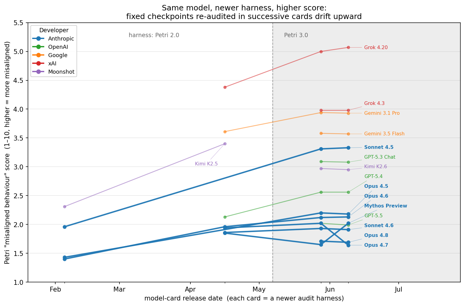
Prediction: newer audits will eventually saturate on older models on the appropriate mix of scenarios. Our model predicts that as monitoring capability rises, observability on older models with fixed $e$ will rise monotonically (and generally smoothly) toward 1. Note that observability is the fraction of misbehaviour caught in AI development contexts. Thus we do not necessarily expect Petri misalignment scores for older models will saturate before those scores saturate on newer models, because new versions of Petri might introduce an ever larger number of contexts that are unrepresentative of vintage AI development with vintage models. The specific prediction is that audits will saturate for older models when confined to a representative, age appropriate sample of development contexts.

Prediction: observability should be relatively weak near the cutting edge. Our model is predicated on the assumption that newer models are better at actively subverting monitoring, and that deployments at the edge of AI capability are harder to monitor. This assumption also implies that leading models deployed on problems that have just been brought into their range of capabilities will have the worst rate of observability, and will be the domains where observability rises most sharply as newer harnesses develop.

Prediction: sharp alignment failures produce a visible hump. As discussed in our analysis of AI-2027, reduced observability from new uncooperative labour happens at a lag from that behaviour being introduced. Thus sudden increases in uncooperative labour will cause visible humps in observed misbehaviour.

Prediction: given no policy change, the observed misbehaviour trend will curve up. Currently, human labour dominates AI production and so the most important source of uncooperative AI behaviour is leakage from human labour. At high rates of automation we will see uncooperative behaviour from two important sources: leakage from cooperative AI labour and self-propagation of existing uncooperative labour. Under our central estimate that leakage from AI labour occurs at about the same rate as the human leakage it displaces ($k_{cu}=k_{hu}$), swapping one for the other roughly cancels. What does not cancel is self-propagation of the uncooperative pool: it grows with the pool itself. Even if there is no relative gain in uncooperative behaviour, as humans dilute the AI labour pool less the uncooperative component will still come to be more important, so the production rate for uncooperative labour can only rise compared to today. Thus, given no changes in effort to detect and suppress misbehaviour, we predict that the trend in observed misbehaviour will bend upwards somewhat in the future. If this is a successful prediction of the model, it will probably be accompanied by findings of transmission of AI misbehaviour between models, scaffolds or sessions, because the bend is mediated by increasing importance of transmission.

Conclusion

The dream motivating this work is an early warning system for loss of control — a monitor that turns existing efforts to monitor the safety of frontier AI into predictions of loss-of-control risk, and that helps to identify the most helpful policy levers. We think a useful version of that is feasible. Several of this model's weaknesses look addressable: better estimates of observability and of the true uncooperative rate seem well within reach, while others — self-propagation, or how leakage behaves as capability grows — are harder. While progress looks possible here too, we acknowledge they are entangled with long-running debates unlikely to be decisively settled soon. Lack of consensus on a parameter is not fatal to the modelling effort; disagreement can be captured by broad sampling distributions - not an ideal solution, because risk-based arguments in the face of a lack of consensus are not reliably persuasive to decision makers, but an epistemically credible solution nonetheless. As a proof of concept, then, we think this work is encouraging, and we think the approach can be carried substantially further.

Setting aside the question of what this approach could deliver in the future, we can ask: what does it deliver today? If the results are taken at face value, two policy takeaways stand out. First, safety looks under-invested: the central path is high-risk, and the uncooperative behaviour we model is undesirable on almost any view of how much authority AI systems should hold. Our crude approach suggests around a three-fold increase in safety investment, with, of course, all the caveats we've presented. Second, and more robustly — because it leans less on our specific parameter choices — it is worth cultivating the ability for the AI industry to change course quickly: ensuring that signals of rising risk propagate efficiently through industry and policy making bodies, and that the relevant actors can respond rapidly and forcefully when adverse signals arrive. The model supports this because dangerous transitions rarely stay hidden — except where change is very gradual, observed misbehaviour moves with the truth — and we buy ourselves a significant amount of safety if we are positioned to respond to these signals when they arise.

AI usage note

This document was primarily authored and directed by David Johnston, with substantial AI assistance (Claude Opus/Fable and the latest version of ChatGPT). Broadly speaking, the model structure was specified by David, and most key assumptions that it encoded were surfaced and evaluated by David, while derivations (such as the transformation to the $\sigma$-clock) and implementations (like the basin explorer, and the sensitivity analyses) were handled by AI. Mathematical requests were handled exclusively by ChatGPT, while other tasks were shared. Many sections were drafted by AI but most, if not all, were rewritten by David. AI assistants were often consulted for feedback on choices, and its feedback was impactful in maybe 10-25% of instances. Both David and AI assistants contributed references and data sources for estimation.

Appendices

Appendix: nonuniform leakage and self-propagation

In our model there are two pools of AI labour, cooperative and uncooperative, and we define each with two-part definitions: a tendency to cooperate/undermine supervision, and a tendency to maintain this tendency. In reality, cooperative behaviour will vary in the degree of behaviour preservation it exhibits, as will uncooperative behaviour. Suppose we have a pool of uncooperative behaviour where half has a very weak behavioural preservation and half has very strong behavioural preservation. Then if we roll the clock forward the strong behavioural preservation component will replicate more effectively than the weak preservation component and - neglecting other sources of uncooperative behaviour - in the next generation, more than half of this pool will have strong behavioural preservation tendencies. In turn, this means that the whole pool will become more effective at self-replication. Thus on this more realistic picture, we won't have a constant $k_{uu}$ pool replication term.

A relatively simple way to address this issue is to increase the number of pools available; rather than a single $A_{c}$ an $A_u$, we have sequences $A^i_u$ and $A^i_c$, $i\in \lbrace 1,2,3,4,5\rbrace$, such that $A^1_c$ has quite weak behavioural preservation tendencies and $A^5_c$ has quite strong tendencies, each with their own replication $k_{x^ix^i}$ and cross-leakage $k_{x^ix^j}$ terms. This adds a large number of parameters to the model which need to be calibrated, and calibrating them is conceptually difficult. Nevertheless, it may be an important upgrade to the model's representational capability.

Note that cross-leakage terms (like $k_{u_1u_2}$) can capture intuitively important processes: suppose it is straightforward for a determined attacker to poison an important dataset so that the next generation of models has modified behaviour in some non-trivial fraction of examples; say, with $1000 of effort they can control 0.01% of responses. However, the control they exercise is crude; the responses they've influenced do not themselves mount similarly effective attacks in their own environment. This can be modeled as "leakage" (or imperfect propagation) from a high-propagation uncooperative class $u_1$ to a lower-propagation but still uncooperative class $u_2$. Plausibly, processes like this are common and importantly determinative of the system dynamics. Note that self-propagation does not necessarily leak to classes that propagate less effectively; plausibly, a tendency to make plans to tile the universe in paperclips is both relatively easy to pass on (like data poisoned behaviours) and effective at self-propagation. The decomposition can help to characterise the process, but it doesn't clearly point towards higher safety or higher risk.

There's an analogy for this in epidemiology. In a textbook SIR model the infectious compartment is a single pool with a constant per-capita recovery rate $\gamma$. That assumption is memoryless: an individual's chance of recovering in the next instant does not depend on how long they have already been infectious, which forces the infectious period to be exponentially distributed — its mode is at zero, its coefficient of variation is one, and it has a long tail. Real infectious periods look nothing like this; they are peaked around a mean. The standard remedy — the "linear chain trick" — is essentially the move proposed above: replace the single compartment with a chain $I_1\to\dots\to I_n$, each substage with rate $n\gamma$. The total time to traverse the chain is then Erlang (a gamma with integer shape) rather than gamma distributed. In epidemiology, multi-stage models tend to fit outbreak data substantially better than the single-exponential default (Wearing, Rohani & Keeling 2005). The same refinement applies to the detect-and-fix sequencing on the suppression side: making the stages a novel failure mode passes through (arrives uncovered → observed → fixed → intercepted) explicit compartments would be the linear-chain version of the $m$-vs-$e$ stock race the current model runs in aggregate.

The cost is that splitting labour pools out by different levels of self-propagating capability will call for additional parameters, many of which are not well characterised by available data. This may well be a cost worth paying for a model that better reflect the key dynamics, but it adds to the estimation and communication burden.

Volatile self-propagation raises risk. Another way that self-propagation and leakage can vary that our model neglects is that it can be volatile in time. There may simply be times where there are better opportunities for uncooperative AI to propagate, and others when the opportunities are worse. For example, a novel propagation method could be discovered which gives a transient opportunity for effective propagation until its respective channel is blocked. This kind of heterogeneity has a clear qualitative consequence: it raises the risk of loss of control. Temporary excursions into more cooperative-dominant regimes do not significantly increase safety, while temporary excursions into more uncooperative-dominant regimes raise risks of permanent loss of control.

An exploratory analysis of this effect — sampling the same ensemble as our headline results and classified on the same 10% line — suggests it is modest for small, light-tailed volatility and important for large, heavy-tailed volatility. Adding time-variation to self-propagation and leakage lowers the fraction of worlds that stay below the 10% high-risk line from 35% to about 29% (light-tailed) or 25% (heavy-tailed) at moderate volatility (20%), and to 27% / 20% at high volatility (40%).

Our model has serious limitations for this purpose: as we have discussed, we don't think it an especially good model of loss of control, which is why we chose to analyse excursions above 10% uncooperative share rather than full takeover. However, volatility matters because it can increase the chance of a discrete loss of control event occurring, so to properly handle volatility we would need a model that credibly handles loss of control events (at least probabilistically).

Appendix: why takeoff speed drops out

The model rests on the assumption that changes in $A_c$ and $A_u$ can be factored into a common time-dependent component $\Lambda(t)$ and allocation functions that depend only on the shares:

\[ \dot A_c = \Lambda(t)\,A\,F_c(q_u,q_h,O), \qquad \dot A_u = \Lambda(t)\,A\,F_u(q_u,q_h,O). \]

The common factor $\Lambda A$ carries everything about how fast the pool is compounding; the $F$'s carry everything about how new production is split, and depend on time only through the shares. The content of the assumption lies in the $F$'s, not in $\Lambda$: $\Lambda $ may depend on time, on $A$, even on the shares themselves — what we assume is that once a single common scale is factored out, the residual split is a function of the shares alone.

Two consequences follow. First, adding the two equations,

\[ \dot A = \dot A_c + \dot A_u = \Lambda A\,(F_c + F_u) = \Lambda A\,F, \qquad F := F_c + F_u, \]

so the clock $\sigma = \log(A/A_0)$ advances at

\[ \dot\sigma = \frac{\dot A}{A} = \Lambda F. \]

Second, for the uncooperative share $q_u = A_u/A$, the quotient rule gives

\[ \dot q_u = \frac{\dot A_u}{A} - q_u\,\frac{\dot A}{A} = \Lambda\,(F_u - q_u F), \]

and re-expressing the rate of change per unit of $\sigma$ rather than per unit of time,

\[ q_u' \;=\; \frac{dq_u}{d\sigma} \;=\; \frac{\dot q_u}{\dot\sigma} \;=\; \frac{\Lambda\,(F_u - q_u F)}{\Lambda F} \;=\; \frac{F_u}{F} - q_u. \]

The common factor $\Lambda$ divides out, top and bottom — and that is the whole trick. It has two parts: because $\Lambda$ is common to both cores, and also sets the clock rate, its magnitude — the takeoff speed — cancels; and because the $F$'s depend on the shares alone, what remains is an autonomous system in $\sigma$. A fast takeoff and a slow takeoff trace the same curve through share-space; only the calendar rate at which they traverse it differs. The cooperative share is just $A_c/A = 1-q_u$, so it needs no equation of its own.

For the fixed human pool $q_h=H_0/A$, we have $\dot H_0=0$, so

\[ \dot q_h = -q_h\,\frac{\dot A}{A} = -q_h\,\Lambda F. \]

Dividing by $\dot\sigma=\Lambda F$ gives

\[ q_h'=-q_h. \]

The same quotient-rule step gives the monitoring and evasion equations. Assume

\[ \dot M = \Lambda A F_m, \qquad \dot E = c_0\,\dot A + \Lambda A\,a_{\mathrm{E/M}}c_mq_u. \]

Monitoring is produced by labour, so it is a production flow like the pools themselves. Evasion splits in two: active evasion is a production flow, but the passive part accrues with automation growth itself — each unit of new automation ships with $c_0$ units of novel failure surface, $dE_{\text{passive}} = c_0,dA$, however the unit was produced. (Both forms keep the σ-clock: any term proportional to $\Lambda$ cancels when we divide by $\dot\sigma$. A passive term pegged to calendar time would not cancel, and would silently reintroduce the takeoff rate.)

For $m=M/A$,

\[ \dot m = \frac{\dot M}{A}-m\,\frac{\dot A}{A} = \Lambda F_m - m\,\Lambda F = \Lambda(F_m-mF). \]

Dividing by $\dot\sigma=\Lambda F$ gives

\[ m'=\frac{F_m}{F}-m. \]

Likewise, for $e=E/A$, using $\dot A/A=\Lambda F$,

\[ \dot e = \frac{\dot E}{A}-e\,\frac{\dot A}{A} = c_0\,\Lambda F+\Lambda\,a_{\mathrm{E/M}}c_mq_u-e\,\Lambda F = \Lambda\left(c_0F+a_{\mathrm{E/M}}c_mq_u-eF\right), \]

and therefore

\[ e'=c_0+\frac{a_{\mathrm{E/M}}c_mq_u}{F}-e=\frac{F_e}{F}-e, \qquad F_e:=c_0F+a_{\mathrm{E/M}}c_mq_u. \]

Appendix: how the Monte-Carlo figures are sampled

The Monte-Carlo results in this post — the plausible-futures bands, the fire-alarm curves, and the path statistics quoted from them — are drawn from a single ensemble. Seven parameters are drawn independently ("log-uniform" means uniform in log space), and the draws are then filtered by a drift condition described below:

parameter	sampled	central
AI leakage $k_{cu}$	log-uniform on $[0.006,,0.22]$ (82% of draws), with a thin tail log-uniform on $[0.22,,0.95]$ (18%)	0.062
human leakage $k_{hu}$	log-uniform on $[0.045,,0.085]$	0.062
evasion vs monitoring $a_{\mathrm{E/M}}$	log-uniform on $[0.73,,5.48]$ (geometric mean 2)	2
self-propagation $k_{uu}$	uniform on $[0.85,,1.35]$	1
present observability $O(0)$	uniform on $[0.30,,0.90]$	0.5
long-run observability dial $\Omega_\infty$	uniform in log-odds on $[0.05,,0.95]$	0.5
AI vs human at monitoring $a_{\mathrm{AI/H}}$	log-uniform on $[1/3,,3]$	1

Uniform distributions are crude, but they're simple and offer broad coverage of the estimated ranges. Better functional forms are possible.

Present observability and long-run observability are sampled independently then draws where present rate of observability change is greater than 10 pp per year are rejected. This makes present observability informative about long-run observability, but only weakly so. Increasing the observability drift limit to 20 pp per year has little effect on results.

A tail is added to $k_{cu}$ to alignment-is-very-hard worlds (leakage approaching 1) in play without letting them dominate; $k_{hu}$ stays close to its measured present-day value, sampled independently of $k_{cu}$ even though the central calibration sets the two equal.

Observability productivity is set as follows. First, the stocks are initialised so that $O_{\mathrm{obs}}(0)=O(0)$, with the share of fixed issues given by $\varphi=\rho/(1+\rho)$: only stock ratios matter for observability, so we gauge today's documented stock to one unit, $b_0+s_0=1$, split at the fix-pipeline steady state ($b_0=\tfrac{1}{1+\rho}$, $s_0=\tfrac{\rho}{1+\rho}$), and set the evasion stock to $e_0=1/O(0)-1$.

Second, $c_m$ is set by the assumption that new behavioural issues are currently being documented at the same rate as fixes are implemented — the documented-issue pipeline is stationary today, $b'(0)=s'(0)=0$, which in this gauge forces the monitoring inflow to match total production, $F_m(0)/F(0)=1$. Since $F_m=c_m\big((1-q_u)+q_h/a_{\mathrm{AI/H}}\big)$, this backs out

\[ c_m=\frac{F(0)}{(1-q_{u,0})+q_{h,0}/a_{\mathrm{AI/H}}}, \qquad F(0)=(1-q_{u,0})+q_{h,0}+k_{uu}q_{u,0}-\delta\,O_{\mathrm{fix},0}\big(L_{k,0}+k_{uu}q_{u,0}\big), \]

with $O_{\mathrm{fix},0}=\varphi,O(0)$ and $L_{k,0}=k_{cu}(1-q_{u,0})+k_{hu}q_{h,0}$. At central parameters this gives $c_m\approx1.0$; across the sampled $a_{\mathrm{AI/H}}$ range it runs $\approx0.37$–$2.3$. Because today's monitoring labour is mostly human, worlds with different $a_{\mathrm{AI/H}}$ describe the same observed present but different futures. Finally, $c_0$ follows from the long-run-dial formula in the parameter table, so the sampled $\Omega_\infty$ is enforced relative to the backed-out $c_m$. The balance assumption is one of convenience (the Petri audits and the OpenAI deception series point in opposite directions on it): relaxing it by 30–60% in either direction moves the headline statistics by only a few points, because the drift condition absorbs the observable consequences.

Everything else is held at its central value ($\delta=0.7$, $\rho=1.27$, $\gamma=1.75$, $q_{u,0}=5%$, $q_{h,0}=5$).

Trajectories are integrated far beyond the plotted window (to $\sigma=220$), and a run is classified contained if its final uncooperative share stays below the 10% line. The plausible-futures figure uses 260 draws; each band is the 7.5th–92.5th percentile range (an 85% interval) with a median line, computed separately for contained and high-risk runs. The fire-alarm curves use 900 draws from the same distributions; at each capability level every path is classified by whether its observed misbehaviour rate sits at or below today's central observed level (≈2.5%, held flat), and the curves report the share of contained outcomes within each class, against the ensemble base rate. A fixed random seed makes the figures exactly reproducible. The outcome map and the crux figures are not sampled: they are deterministic sweeps of one or two parameters with everything else held central.